Quick Start Guide: Heuristic Classifiers
In this example we will use classifiers from Heuristics on the banknote authentication dataset. First we load in the data and split into training and test datasets:
using CSV, DataFrames
df = DataFrame(CSV.File("data_banknote_authentication.txt",
    header=[:variance, :skewness, :curtosis, :entropy, :class]))
1372×5 DataFrame
Row │ variance skewness curtosis entropy class
│ Float64 Float64 Float64 Float64 Int64
──────┼─────────────────────────────────────────────────
1 │ 3.6216 8.6661 -2.8073 -0.44699 0
2 │ 4.5459 8.1674 -2.4586 -1.4621 0
3 │ 3.866 -2.6383 1.9242 0.10645 0
4 │ 3.4566 9.5228 -4.0112 -3.5944 0
5 │ 0.32924 -4.4552 4.5718 -0.9888 0
6 │ 4.3684 9.6718 -3.9606 -3.1625 0
7 │ 3.5912 3.0129 0.72888 0.56421 0
8 │ 2.0922 -6.81 8.4636 -0.60216 0
⋮ │ ⋮ ⋮ ⋮ ⋮ ⋮
1366 │ -4.5046 -5.8126 10.8867 -0.52846 1
1367 │ -2.41 3.7433 -0.40215 -1.2953 1
1368 │ 0.40614 1.3492 -1.4501 -0.55949 1
1369 │ -1.3887 -4.8773 6.4774 0.34179 1
1370 │ -3.7503 -13.4586 17.5932 -2.7771 1
1371 │ -3.5637 -8.3827 12.393 -1.2823 1
1372 │ -2.5419 -0.65804 2.6842 1.1952 1
1357 rows omittedX = df[:, 1:4]
y = df[:, 5]
(train_X, train_y), (test_X, test_y) = IAI.split_data(:classification, X, y,
seed=1)Random Forest Classifier
We will use a GridSearch to fit a RandomForestClassifier with some basic parameter validation:
grid = IAI.GridSearch(
    IAI.RandomForestClassifier(
        random_seed=1,
    ),
    max_depth=5:10,
)
IAI.fit!(grid, train_X, train_y)
All Grid Results:
Row │ max_depth train_score valid_score rank_valid_score
│ Int64 Float64 Float64 Int64
─────┼───────────────────────────────────────────────────────
1 │ 5 0.896915 0.866758 6
2 │ 6 0.938223 0.899417 5
3 │ 7 0.956856 0.912661 4
4 │ 8 0.963755 0.920417 3
5 │ 9 0.965845 0.920693 2
6 │ 10 0.966141 0.921069 1
Best Params:
max_depth => 10
Best Model - Fitted RandomForestClassifierWe can make predictions on new data using predict:
IAI.predict(grid, test_X)412-element Vector{Int64}:
0
0
0
0
0
0
0
0
0
0
⋮
1
1
1
1
1
1
1
1
1We can evaluate the quality of the model using score with any of the supported loss functions. For example, the misclassification on the training set:
IAI.score(grid, train_X, train_y, criterion=:misclassification)1.0Or the AUC on the test set:
IAI.score(grid, test_X, test_y, criterion=:auc)0.9999761376381036We can also look at the variable importance:
IAI.variable_importance(IAI.get_learner(grid))4×2 DataFrame
Row │ Feature Importance
│ Symbol Float64
─────┼──────────────────────
1 │ variance 0.549464
2 │ skewness 0.251803
3 │ curtosis 0.143985
4 │ entropy 0.0547478XGBoost Classifier
We will use a GridSearch to fit an XGBoostClassifier with some basic parameter validation:
grid = IAI.GridSearch(
    IAI.XGBoostClassifier(
        random_seed=1,
    ),
    max_depth=2:5,
    num_round=[20, 50, 100],
)
IAI.fit!(grid, train_X, train_y)
All Grid Results:
Row │ num_round max_depth train_score valid_score rank_valid_score
│ Int64 Int64 Float64 Float64 Int64
─────┼──────────────────────────────────────────────────────────────────
1 │ 20 2 0.909192 0.886487 12
2 │ 20 3 0.973674 0.92655 11
3 │ 20 4 0.987791 0.941853 9
4 │ 20 5 0.989819 0.936374 10
5 │ 50 2 0.984743 0.966999 2
6 │ 50 3 0.995245 0.954592 5
7 │ 50 4 0.996033 0.952682 6
8 │ 50 5 0.996368 0.949697 8
9 │ 100 2 0.995576 0.982432 1
10 │ 100 3 0.996672 0.958094 3
11 │ 100 4 0.99691 0.957024 4
12 │ 100 5 0.997079 0.952448 7
Best Params:
num_round => 100
max_depth => 2
Best Model - Fitted XGBoostClassifierWe can make predictions on new data using predict:
IAI.predict(grid, test_X)412-element Vector{Int64}:
0
0
0
0
0
0
0
0
0
0
⋮
1
1
1
1
1
1
1
1
1We can evaluate the quality of the model using score with any of the supported loss functions. For example, the misclassification on the training set:
IAI.score(grid, train_X, train_y, criterion=:misclassification)1.0Or the AUC on the test set:
IAI.score(grid, test_X, test_y, criterion=:auc)0.9999284129143106We can also look at the variable importance:
IAI.variable_importance(IAI.get_learner(grid))4×2 DataFrame
Row │ Feature Importance
│ Symbol Float64
─────┼──────────────────────
1 │ variance 0.59187
2 │ skewness 0.215287
3 │ curtosis 0.153911
4 │ entropy 0.0389316We can calculate the SHAP values:
s = IAI.predict_shap(grid, test_X)
s[:shap_values][1]
412×4 Matrix{Float64}:
3.54498 3.22913 -2.00503 0.3945
0.728945 -1.46553 2.35883 0.735524
3.39881 3.29186 -2.13044 0.300303
2.95136 -2.37941 2.52937 0.648339
1.1021 3.35015 -1.98985 0.507956
4.3507 -1.7485 0.930799 -0.612113
4.09464 -1.62499 1.86802 -0.612113
4.34745 -0.151717 -0.125396 -0.313408
3.2987 3.23863 -2.67317 0.300303
-0.15059 -1.10272 2.54168 -0.638055
⋮
1.17481 -0.609447 -4.14658 0.41376
-2.12014 -2.18583 0.292272 -0.725072
-0.380289 -1.71014 -1.14518 -0.673723
1.35037 -0.504165 -3.06564 -0.485776
1.4018 -0.716085 -3.27848 0.507956
-0.480185 -0.789143 -3.00252 0.41376
-2.86904 -0.471602 -1.27742 0.460438
-1.79681 -1.81585 1.27945 -0.682587
-3.11327 -1.48426 1.06169 -0.700595We can then use the SHAP library in Python to visualize these results in whichever way we prefer. For example, the following code creates a summary plot:
using PyCall
shap = pyimport("shap")
shap.summary_plot(s[:shap_values][1], Matrix(s[:features]), names(s[:features]))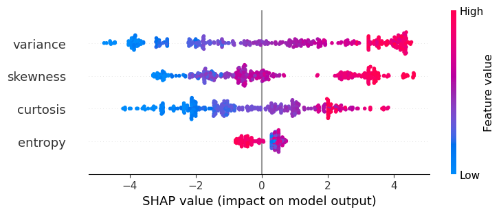
GLMNet Classifier
We can use a GLMNetCVClassifier to fit a GLMNet model using cross-validation:
lnr = IAI.GLMNetCVClassifier(
    random_seed=1,
    n_folds=10,
)
IAI.fit!(lnr, train_X, train_y)
Fitted GLMNetCVClassifier:
Constant: 5.28597
Weights:
curtosis: -3.73106
entropy: -0.345243
skewness: -2.99037
variance: -5.54063
(Higher score indicates stronger prediction for class `1`)We can access the coefficients from the fitted model with get_prediction_weights and get_prediction_constant:
numeric_weights, categoric_weights = IAI.get_prediction_weights(lnr)
numeric_weights
Dict{Symbol, Float64} with 4 entries:
:curtosis => -3.73106
:skewness => -2.99037
:entropy => -0.345243
:variance => -5.54063categoric_weightsDict{Symbol, Dict{Any, Float64}}()IAI.get_prediction_constant(lnr)5.28596534We can make predictions on new data using predict:
IAI.predict(lnr, test_X)412-element Vector{Int64}:
0
1
0
0
0
0
0
0
0
0
⋮
1
1
1
1
1
1
1
1
1We can evaluate the quality of the model using score with any of the supported loss functions. For example, the misclassification on the training set:
IAI.score(lnr, train_X, train_y, criterion=:misclassification)0.9864583333333333Or the AUC on the test set:
IAI.score(lnr, test_X, test_y, criterion=:auc)0.9999522752762073We can also look at the variable importance:
IAI.variable_importance(lnr)4×2 DataFrame
Row │ Feature Importance
│ Symbol Float64
─────┼──────────────────────
1 │ skewness 0.352005
2 │ curtosis 0.320189
3 │ variance 0.313268
4 │ entropy 0.0145371