Optimal Prescription for Diabetes Management
In this example, we aim to learn an optimal diabetes management policy from observational data. We use a cleaned dataset based on an Electronic Medical Records database (for patient confidentiality reasons, we cannot share the dataset publically).
We show how Optimal Policy Trees can be used to inform interpretable diabetes management policies. In particular, we demonstrate that by treating treatments as combination of numeric doses instead of categorical, mutually independent options, we achieve much better prescription outcomes in unseen data.
This case is a simplified version of what is presented in Amram et al. 2020. At the end of the case, we describe some of the modifications done in the paper to make the setting more realistic.
Preparing the dataset
First, we load the prepared data and separate out the features, treatments, and outcomes (HbA1c, the lower the better). The treatments are coded as a vector of three numbers, corresponding to the amount in each of tree distinct drug classes: insulin, metformin, and oral drugs. We then separate the data into training and testing.
using CSV, DataFrames, CategoricalArrays
using Statistics
using CategoricalArrays

df = CSV.read("diabetes.csv", DataFrame)
transform!(df, [:raceBucket, :SEX_CD] .=> categorical, renamecols=false)

train_df = df[df.train, :]
test_df = df[(!).(df.train), :]
train_X = train_df[:, 1:23]
train_T = train_df[:, 24:26]
train_y = train_df[:, :x1]
test_X = test_df[:, 1:23]
test_T = test_df[:, 24:26]
test_y = test_df[:, :x1]
Because not all treatment combinations are feasible from a medical perspective, we need to also load in the candidate prescription options:
candidates = CSV.read("candidates.csv", DataFrame)13×3 DataFrame
Row │ ins met oral
│ Float64 Float64 Float64
─────┼───────────────────────────
1 │ 0.0 0.0 2.0
2 │ 0.0 1.0 1.0
3 │ 0.0 0.0 1.0
4 │ 1.0 1.0 1.0
5 │ 0.0 1.0 0.0
6 │ 1.0 0.0 1.0
7 │ 0.0 0.0 3.0
8 │ 0.1 0.1 0.1
9 │ 0.0 0.0 0.0
10 │ 0.0 1.0 2.0
11 │ 1.0 0.0 0.0
12 │ 1.0 1.0 0.0
13 │ 1.0 0.0 2.0Optimal Policy Trees with Multiple Numeric Treatments
Optimal Policy Trees separate the tasks of estimating the counterfactuals and learning the prescription policy. This means that in order to train the tree, we require the input of a reward matrix - that is, the outcome under each of the possible policies for each sample in the data.
The first step is to create the reward matrix. One of the key advantages that Optimal Policy Trees has over Optimal Prescriptive Trees and regress-per-treatment-and-compare methods is that it does not need to onehot-encode treatments into distinct options. In other words, it preserves the order of treatment intensities and hence has a sense of meaningful similarity. For example, we have that "insulin + metformin" (encoded as [1,1,0]) is closer to "insulin + metformin + oral drug" ([1,1,1]) than "2 oral drugs" ([0,0,2]). Note that this is not the case if we have to onehot-encode the treatments into 13 distinct options.
Since the treatments are numeric, we use IAI.NumericRegressionRewardEstimator to estimate the counterfactual reward matrix under each candidate treatment option:
seed = 1
reward_lnr = IAI.NumericRegressionRewardEstimator(
    outcome_estimator=IAI.RandomForestRegressor(),
    outcome_insample_num_folds=2,
    propensity_estimator=IAI.RandomForestRegressor(),
    propensity_insample_num_folds=2,
    propensity_min_value=0.001,
    reward_estimator=:doubly_robust,
    estimation_kernel_bandwidth=2,
    reward_kernel_bandwidth=1,
    random_seed=seed,
)
train_predictions, train_score = IAI.fit_predict!(
      reward_lnr, train_X, train_T, train_y, candidates)
train_rewards = train_predictions[:reward]
train_score[:outcome]
Dict{String, Float64} with 13 entries:
"[1.0,1.0,0.0]" => 0.414331
"[0.0,1.0,0.0]" => 0.542481
"[1.0,0.0,1.0]" => 0.421292
"[1.0,0.0,0.0]" => 0.479701
"[0.0,0.0,1.0]" => 0.52907
"[0.0,1.0,2.0]" => 0.259584
"[1.0,0.0,2.0]" => 0.299357
"[0.0,1.0,1.0]" => 0.419445
"[0.0,0.0,2.0]" => 0.47051
"[0.0,0.0,3.0]" => 0.207696
"[1.0,1.0,1.0]" => 0.110443
"[0.0,0.0,0.0]" => 0.476753
"[0.1,0.1,0.1]" => 0.467101train_score[:propensity]Dict{String, Float64} with 13 entries:
"[1.0,1.0,0.0]" => 0.848864
"[0.0,1.0,0.0]" => 0.875902
"[1.0,0.0,1.0]" => 0.760202
"[1.0,0.0,0.0]" => 0.86626
"[0.0,0.0,1.0]" => 0.821753
"[0.0,1.0,2.0]" => 0.820372
"[1.0,0.0,2.0]" => 0.610685
"[0.0,1.0,1.0]" => 0.827607
"[0.0,0.0,2.0]" => 0.663629
"[0.0,0.0,3.0]" => 0.726535
"[1.0,1.0,1.0]" => 0.784474
"[0.0,0.0,0.0]" => 0.886931
"[0.1,0.1,0.1]" => 0.918676The R-squared scores of the internal estimators are reasonable, giving us confidence that the value for estimation_kernel_bandwidth is fine and that there is sufficient signal in the data to use for making prescriptions.
Let's now tune the reward_kernel_bandwidth. Following the guide to bandwidth tuning, we inspect the tuned bandwidth based on a series on input values:
using Plots
in = 0.5:0.5:5
out = IAI.tune_reward_kernel_bandwidth(reward_lnr, train_T, train_y,
                                       train_predictions, in)
plot(in, out, label=nothing)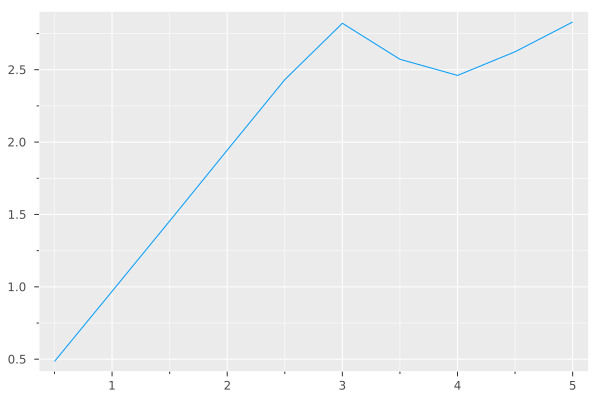
The figure does not show a plateau or peak, so there is no real guidance as to the best bandwidth to use. As per the tuning guide, in such cases a good rule of thumb is to set the bandwidth to the same value as the estimation_kernel_bandwidth:
reward_lnr.reward_kernel_bandwidth = 2
train_predictions = IAI.predict_reward(reward_lnr, train_T, train_y,
                                       train_predictions)
train_rewards = train_predictions[:reward]
With the reward matrix as the input in addition to the features, we can now learn an Optimal Policy Tree:
policy_grid = IAI.GridSearch(
    IAI.OptimalTreePolicyMinimizer(
      random_seed=seed,
      minbucket=10,
    ),
    max_depth=1:5,
)
IAI.fit!(policy_grid, train_X, train_rewards)We obtain a tree that splits using information such as time since diagnosis, age, BMI, and past HbA1c. For example, we would recommend metformin monotherapy if BMI is below 39 and past HbA1c is below 7. This is consistent with the medical knowledge that this is one of the least intensive treatment options. In contrast, we would prescribe insulin plus metformin, or a combination of three when past HbA1c is high.
Evaluation in the Test Set
Since we do not know the true outcome under each treatment in the test set, we need another procedure for estimation so we can evaluate in the test set. We use the same procedure as before to estimate the revenue under each candidate treatment, but now on the test set:
test_predictions, test_score = IAI.fit_predict!(
      reward_lnr, test_X, test_T, test_y, candidates)
test_rewards = test_predictions[:reward]
test_score[:outcome]
Dict{String, Float64} with 13 entries:
"[1.0,1.0,0.0]" => 0.394017
"[0.0,1.0,0.0]" => 0.480555
"[1.0,0.0,1.0]" => 0.278825
"[1.0,0.0,0.0]" => 0.367026
"[0.0,0.0,1.0]" => 0.437722
"[0.0,1.0,2.0]" => 0.271445
"[1.0,0.0,2.0]" => 0.512792
"[0.0,1.0,1.0]" => 0.323137
"[0.0,0.0,2.0]" => 0.439781
"[0.0,0.0,3.0]" => 0.124681
"[1.0,1.0,1.0]" => 0.477906
"[0.0,0.0,0.0]" => 0.481497
"[0.1,0.1,0.1]" => 0.49046test_score[:propensity]Dict{String, Float64} with 13 entries:
"[1.0,1.0,0.0]" => 0.845982
"[0.0,1.0,0.0]" => 0.884052
"[1.0,0.0,1.0]" => 0.77498
"[1.0,0.0,0.0]" => 0.888425
"[0.0,0.0,1.0]" => 0.82715
"[0.0,1.0,2.0]" => 0.857055
"[1.0,0.0,2.0]" => 0.409752
"[0.0,1.0,1.0]" => 0.855677
"[0.0,0.0,2.0]" => 0.742228
"[0.0,0.0,3.0]" => 0.644165
"[1.0,1.0,1.0]" => 0.801384
"[0.0,0.0,0.0]" => 0.898054
"[0.1,0.1,0.1]" => 0.926831Again, the test scores are reasonable, allowing us to trust these values for out-of-sample evaluation. We evaluate the method by calculating the predicted HbA1c outcome under the new diabetes treatment strategy:
outcomes = IAI.predict_outcomes(policy_grid, test_X, test_rewards)
mean(outcomes)
7.67054427And compare to what is being prescribed in reality:
test_T_categorical = Symbol.("[", test_T.ins, ",", test_T.met, ",", test_T.ins, "]")
curr_outcomes = [test_rewards[i, test_T_categorical[i]] for i in 1:length(test_T_categorical)]
mean(curr_outcomes)7.8401704We see that there is a significant reduction of 0.17 in HbA1c under the optimal policy, much higher than a clinically meaningful threshold of 0.05.
Optimal Policy Trees with Categorical Treatments
We mentioned previously the advantage of not having to onehot encode the treatments in Optimal Policy Trees. To verify if there is indeed such an advantage, let's try generating the reward matrix with treatments encoded as distinct categories with IAI.CategoricalRegressionRewardEstimator:
train_T_categorical = string.("[", train_T.ins, ",", train_T.met, ",", train_T.ins, "]")
categorical_reward_lnr = IAI.CategoricalRegressionRewardEstimator(
    propensity_estimator=IAI.RandomForestClassifier(),
    outcome_estimator=IAI.RandomForestRegressor(),
    reward_estimator=:doubly_robust,
    propensity_min_value=0.001,
    random_seed=seed,
)
train_predictions, train_score = IAI.fit_predict!(
      categorical_reward_lnr, train_X, train_T_categorical, train_y)
train_rewards = train_predictions[:reward]
train_score[:outcome]
Dict{String, Float64} with 5 entries:
"[0.0,1.0,0.0]" => 0.521172
"[1.0,0.0,1.0]" => 0.484973
"[1.0,1.0,1.0]" => 0.371429
"[0.0,0.0,0.0]" => 0.557221
"[0.1,0.1,0.1]" => 0.340729train_score[:propensity]0.7331914751301537Notice that we have decent scores for both the propensity estimator and the outcome estimators. Let's now train an Optimal Policy Tree:
categorical_policy_grid = IAI.GridSearch(
    IAI.OptimalTreePolicyMinimizer(
      random_seed=seed,
    ),
    max_depth=1:5,
)
IAI.fit!(categorical_policy_grid, train_X, train_rewards)Similarly, we can look at the outcome under the prescription in test data:
outcomes = IAI.predict_outcomes(categorical_policy_grid, test_X, test_rewards)
mean(outcomes)7.72813084The results are worse than Optimal Policy Tree with numeric treatments, while still better than the current prescription. This suggests that by encoding the treaments as distinct categorical options, we lose the relationship between different treatments when estimating the reward matrix, and therefore we do not obtain as strong a policy tree in the end.
Optimal Prescriptive Trees with Categorical Treatments
Similarly, with categorical treatments, we can train an Optimal Prescriptive Tree (which is not possible with numeric treatments):
prescriptive_grid = IAI.GridSearch(
    IAI.OptimalTreePrescriptionMinimizer(
      random_seed=seed,
    ),
    max_depth=1:5,
)
IAI.fit!(prescriptive_grid, train_X, train_T_categorical, train_y)We similarly evaluate the outcomes in test data:
pred_treatments, _ = IAI.predict(prescriptive_grid, test_X)
pred_outcomes = [test_rewards[i, pred_treatments[i]] for i in 1:length(pred_treatments)]
mean(pred_outcomes)7.92357198Which is worse than the results from both Optimal Policy Trees approaches and also worse than the current treatments.
Additional Modifications
In the paper, we made some adjustments to adapt to the practical considerations in the medical setting. For example, some of the treatments cannot be assigned to a specific patient due to medical reasons (some drugs have contra-indications, some are not allowed based on kidney conditions, or some combinations are some too drastic a change from current therapy, etc.) To incorporate these considerations, we can use the IAI.predict_treatment_rank function to obtain an ordered list of treatments and find the best feasible one from the set.
Another modification made was that sometimes an adjustment should only be made when we have sufficient confidence that the expected improvement is large. We then introduce a threshold delta where change is recommended only if the predicted outcome under the best treatment is better than current one by at least delta. Otherwise, we recommend the person should stay on their current regimen.
The paper additionally compares against regress-and-compare approaches and other baselines and found similar patterns.
Conclusions
This case shows that by using an Optimal Policy Trees approach, we can learn an interpretable policy to recommend treatments for diabetes patients that significantly improves their HbA1c compared to the standard of care.
Comparing against other options, Optimal Policy Trees allow us to directly use the treatments as a combination of numeric doses instead of having to encode them as categorical options. This leads to stronger reward estimates and much better prescribed outcomes in unseen data.