Tree Stability
Decision tree methods carry a reputation for being unstable - small variations in the training process can have large effects on the derived model. This perception of instability is not unfounded, as CART and other greedy tree-based models are particularly susceptible to the following instability issues:
- small variations in the training data can lead to the greedy algorithm making different decisions near the top of the tree, resulting in vastly different solutions
- the cost-complexity algorithm for tree pruning (used for tuning the complexity parameter
cp) has very high variance, and can give vastly different results
Fortunately, Optimal Trees are not as susceptible to these issues as greedy tree algorithms: the trees are constructed using global optimization so are not locked into bad decisions early in the training process, and the automatic complexity parameter tuning is significantly more precise than the algorithm used for CART.
However, we still observe that the trained trees may change in response to differences in the training process, such as changes to the training data or parameters (such as using a different random seed). There are a number of reasons this may occur, including:
Instability Source 1:
The training process can be under-optimizing the problem, and so each time we run the trees, we are only seeing a "good" solution, rather than one that is near-optimal. In this case, the instability can often be remedied by adjusting the parameters and their tuning to achieve better and more consistent results.
Instability Source 2:
There can be many high-quality solutions to the problem that have similar performance yet appear structurally different. Any of these solutions has the potential to be returned as the final solution, and additional criteria or human judgement may be useful in choosing between them.
Instability Source 3:
If the training data is changed, the variation in the training data may be sufficiently large that the optimal solution to the new problem is actually significantly different to the original solution. In this case, we may want to explore the tradeoff between the quality of the new solution and proximity to the original solution in order to understand the degree to which the solution should change.
When training Optimal Trees, the algorithm optimizes many different trees from random starting solutions (the number of such trees is controlled by the ls_num_tree_restarts parameter). The training process thus produces multiple candidate solutions, among which the one with the best training objective value is chosen as the final solution. However, the candidate trees can also be analyzed with a number of tools that allow us to understand and explore these sources of instability.
As a case study, we will use these tools to investigate stability of Optimal Classification Trees on the banknote authentication dataset, so we will load in the data and split into training and testing datasets of equal sizes:
using CSV, DataFrames
df = CSV.read("data_banknote_authentication.txt", DataFrame,
              header=[:variance, :skewness, :curtosis, :entropy, :class])
X = df[:, 1:4]
y = df[:, 5]
(train_X, train_y), (test_X, test_y) =
    IAI.split_data(:classification, X, y, seed=1, train_proportion=0.5)
Stability on Fixed Dataset
Firstly, we will analyze the stability of the training procedure on a single fixed dataset. In terms of our instability sources above, this means:
- to investigate Instability Source 1, we should determine if the model is sufficiently well-optimized
- to investigate Instability Source 2, we should determine if there are multiple high-quality solutions to the problem, and if so, explore these solutions
- since we are not changing the training data, Instability Source 3 is not a relevant concern in this setting
This analysis is conducted after training a learner, so we will use a GridSearch to fit an OptimalTreeClassifier:
grid = IAI.GridSearch(
    IAI.OptimalTreeClassifier(random_seed=1),
    max_depth=1:5,
    validation_criterion=:auc,
)
IAI.fit!(grid, train_X, train_y)
lnr = IAI.get_learner(grid)We conduct the stability analysis using StabilityAnalysis, which requires us to pass the trained learner, and optionally a calibration dataset and scoring criterion to use for determining tree similarity. As recommended for classification problems, we use the gini criterion determining the similarity scores, as this typically gives more specific results than the default misclassification.
stability = IAI.StabilityAnalysis(lnr, train_X, train_y, criterion=:gini)We can plot a summary of the analysis using Plots.plot:
using Plots
plot(stability, size=(500, 600))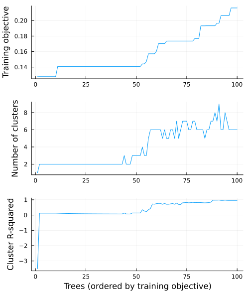
This produces three plots:
Training objective of the different trees
This plot shows the trees found during training, sorted in increasing order of objective value (where a lower objective value is better). This enables us to see how many trees share the same performance during training.
In this case, we see that the best 10 trees have the same objective value, and then the following 40 trees all have a slighter worse value. This gives us evidence against Instability Source 1, as 10% of the candidate trees achieve the optimal objective value. If instead we observed that the optimal objective value was only achieved by very few trees, this would be evidence of under-optimizing, and we might want to increase the value of
ls_num_tree_restartsto increase the stability of the training procedure.Number of clusters present among the best trees
This plot analyzes the similarity of the trees found during training by showing the number of distinct clusters among the best $n$ trees, for each value of $n$. For instance, when we consider the first 25 trees, we see there are two clusters of tree structures, whereas among the best 50 trees, there are three distinct clusters of tree structure.
When we consider the best 10 trees that all have the same optimal objective value, we see that there are two clusters of similar tree structure. This tells us that there are multiple distinct optimal solutions to the problem, and so Instability Source 2 may become an issue. The next plot can help us quantify the extent of this problem.
How much of the space the tree clusters span
This plot gives a sense of how different the clusters of trees are at each step. We do this by measuring how much of the total variation in tree structure across all trees is explained by the clustering of the best $n$ trees. In this case, we see that the first cluster is very different to the second, as evidenced by the large jump in the plot. The clusters are very similar until around the 60th tree, where the plot again begins to climb, eventually approaching full coverage of the space as we include all the trees.
The fact that the first cluster is very different to the second is evidence that Instability Source 2 may be a problem for this dataset, as this means that there are large structural differences among our multiple optimal solutions, so the final tree may change drastically from run to run.
In addition to these plots, we can also explore the results of the analysis quantitatively. The analysis uses the variable importance of features in each tree to measure similarity between tree structures and to cluster the trees, and get_stability_results allows us to extract the trees in order of training objective along with the importance of each feature in the tree:
IAI.get_stability_results(stability)100×6 DataFrame
Row │ train_error tree_index variance skewness curtosis entropy
│ Float64 Int64 Float64 Float64 Float64 Float64
─────┼──────────────────────────────────────────────────────────────────
1 │ 0.127639 38 0.601713 0.395491 0.00279545 0.0
2 │ 0.127677 21 0.615924 0.237532 0.146544 0.0
3 │ 0.127677 22 0.615924 0.237532 0.146544 0.0
4 │ 0.127677 29 0.615924 0.237532 0.146544 0.0
5 │ 0.127677 39 0.615924 0.237532 0.146544 0.0
6 │ 0.127677 55 0.615924 0.237532 0.146544 0.0
7 │ 0.127677 59 0.615924 0.237532 0.146544 0.0
8 │ 0.127677 70 0.615924 0.237532 0.146544 0.0
⋮ │ ⋮ ⋮ ⋮ ⋮ ⋮ ⋮
94 │ 0.206366 36 0.78342 0.185882 0.0306976 0.0
95 │ 0.206366 57 0.78342 0.185882 0.0306976 0.0
96 │ 0.206366 76 0.78342 0.185882 0.0306976 0.0
97 │ 0.21624 87 0.746042 0.195427 0.0585311 0.0
98 │ 0.21624 25 0.764514 0.196132 0.0393544 0.0
99 │ 0.21624 30 0.764514 0.196132 0.0393544 0.0
100 │ 0.21624 100 0.764514 0.196132 0.0393544 0.0
85 rows omittedWe see that the first tree, Tree 38, looks to have a different structure to the trees that immediately follow (Trees 21, 22, 29, etc). Specifically, it uses the curtosis feature very little, unlike the other trees. However, since the training performance is almost identical, Instability Source 1 is unlikely to be an issue here, as we consistently find good solutions to the problem.
Given that the first 10 trees all have approximately the same optimal training performance, we can now examine the structural similarity among these trees to investigate Instability Source 2 . We can use get_cluster_details to summarize the clustering of these 10 trees:
IAI.get_cluster_details(stability, 10)2×5 DataFrame
Row │ train_error_mean variance skewness curtosis entropy
│ Float64 Float64 Float64 Float64 Float64
─────┼───────────────────────────────────────────────────────────
1 │ 0.127639 0.601713 0.395491 0.00279545 0.0
2 │ 0.127677 0.615924 0.237532 0.146544 0.0We can also use get_cluster_distances to get the relative distances between each pair of clusters (this is useful in situations with a larger number of clusters to get a sense of the relative proximity of the clusters):
IAI.get_cluster_distances(stability, 10)2×2 Matrix{Float64}:
0.0 0.214048
0.214048 0.0We can use get_cluster_assignments to see which trees comprise each cluster:
IAI.get_cluster_assignments(stability, 10)2-element Vector{Vector{Int64}}:
[38]
[21, 22, 29, 39, 55, 59, 70, 96, 97]We see that Tree 38 is in its own cluster, and the other trees are all grouped together.
Given this, we might want to inspect how Tree 38 differs to the others. We can use get_tree to construct a new learner that uses the tree at a specified index:
IAI.get_tree(lnr, 38)IAI.get_tree(lnr, 21)We can see that the trees have some structural similarities (e.g. splitting on skewness at 5.1 and then variance at -3.4), but also some differences. The fact that 9/10 of these best 10 trees fall into one cluster might indicate that this solution is more stable and easier to find than Tree 38.
It seems that this problem indeed exhibits Instability Source 2, as there are two different optimal solutions that are equally plausible. In a real application, we might inspect both groups of trees carefully to see if we can learn anything, and if one tree structure might be more appropriate or desirable than the other.
As a final note, we can also generate an interactive visualization that allows us to explore all of the information in the stability analysis using write_html or show_in_browser:
IAI.write_html("stability_analysis.html", stability)The resulting interactive visualization can be viewed here. As with all visualizations, this visualization is also automatically shown inside a Jupyter notebook.
Stability on Changing Dataset
Now, suppose we want to measure the stability of our training procedure when the training dataset is varied. To do this, we can pretend that our test set is a new version of the dataset that we want to use to update our tree. This exposes us to the risk of Instability Source 3, and so we might be interested in understanding whether we can still obtain a solution close to the original solution, or if any changes to the tree structure were driven by actual shifts in the underlying training data.
To get started, we can train a new learner on this new dataset:
new_grid = IAI.GridSearch(
    IAI.OptimalTreeClassifier(random_seed=1),
    max_depth=1:5,
    validation_criterion=:auc,
)
IAI.fit!(new_grid, test_X, test_y)
new_lnr = IAI.get_learner(new_grid)We see that this tree is quite different to the tree in the original learner. To investigate Instability Source 3 and understand if the difference comes from instability in the training process or a shift in the underlying data, we can use variable_importance_similarity to compute the difference between the original tree and each tree in the new learner, and feed this into SimilarityComparison:
deviations = IAI.variable_importance_similarity(lnr, new_lnr, test_X, test_y,
                                                criterion=:gini)
similarity = IAI.SimilarityComparison(lnr, new_lnr, deviations)
We can plot a summary of the analysis using Plots.plot:
using Plots
plot(similarity)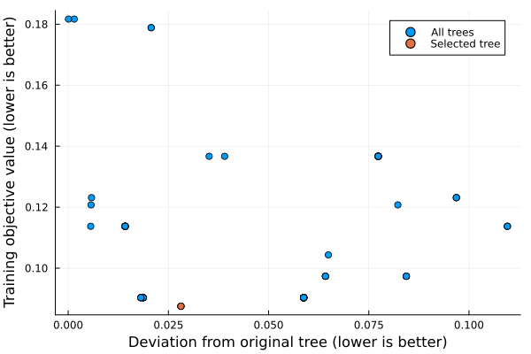
This plot shows the training objective value on the new dataset for all of the trees in the new learner against their similarity to the tree trained on the original dataset. The selected tree in the new learner is indicated in red. We can see that this tree had the lowest objective value on the new dataset, and there were no ties for best solution. There are other trees that are closer in structure to the original tree, but this comes at the expense of tree quality. This indicates that Instability Source 3 is present as a result of a shift in the underlying data, and that the new dataset justifies a tree that is significantly different to the tree trained on the original dataset. If this were not the case (meaning the new data was not sufficiently different to the original dataset), we would expect to see trees with both strong training performance and high similarity to the original tree (in the lower-left of this plot), as the original tree would still be a high-quality solution for this new dataset.
We can get the training objective values with get_train_errors, allowing us to explore the individual trees of interest on the plot. For instance, the following tree is one of the trees on the efficient frontier:
train_errors = IAI.get_train_errors(similarity)
index = findfirst((train_errors .< 0.12) .& (deviations .< 0.01))
IAI.get_tree(new_lnr, index)As we did for stability analysis, we can also generate an interactive visualization that allows us to explore all of the information in the similarity comparison using write_html or show_in_browser:
IAI.write_html("similarity_comparison.html", similarity)The resulting interactive visualization can be viewed here. As with all visualizations, this visualization is also automatically shown inside a Jupyter notebook.