Differences between R and Julia
The IAI R interface matches the Julia API very closely, so you can refer to the Julia documentation for information on most tasks. On this page we note the main differences between the R and Julia interfaces.
Conversion of Julia data types to R
In order to figure out the types to pass to an IAI function from the R interface, you can refer to the equivalent function in the Julia API and translate the types to their R equivalent. Most literal data types convert in a straighforward manner, for example:
Inttointeger(can also pass as a round-numberdouble, e.g.,1.0)Float64todoubleStringtocharacterDicttolist
The following Julia types can be passed as follows:
nothingcan be passed usingNULL- a
Symbolcan be passed as acharacter - a
Vectorcan be passed as an atomicvector - a
Matrixcan be passed as amatrix - a
DataFramecan be passed as adata.frame
Specifying Feature Set in R
We list the R input types for specifying set of features in a dataframe as learner parameters. Refer to IAI.FeatureSet for the Julia equivalence:
| Input Type | Description | Examples |
|---|---|---|
All | Use all columns | list(All = c()) |
Integer or a vector of Integers | Specify indices of columns to use | 1, c(1, 3, 4) |
String or a vector of Strings | Specify names of columns to use | "x1", c("x1", "x3") |
Not | Specify columns not to use | list(Not = 1), list(Not = c("x2", "x4")) |
Between | Specify range of columns to use | list(Between = c("x1", "x4")) |
Interactive Visualizations
The write_html and show_in_browser functions work the same in R as in Julia for saving visualizations to file or displaying in an external browser, respectively. Additionally, visualizations will be automatically shown in the viewer pane when using RStudio, similar to how visualizations are automatically displayed in Jupyter notebooks.
To include data in the tree visualization, the data keyword argument should be passed as an unnamed list:
iai::write_html("tree.html", lnr, data = list(X, y))
Below is an example that shows the equivalent R code for the advanced visualization examples in Julia. In these examples we work with the following tree learner:
We can rename the features with a list that maps from the original names to more descriptive names:
vis_renamed_features <- iai::tree_plot(lnr, feature_renames = list(
  "disp" = "Displacement",
  "hp" = "Horsepower",
  "wt" = "Weight"
))
We can also have a finer-grained control of what is displayed for each node, such as adding summary statistics. We create a list of lists with the parameters controlling what you want to show in each node and pass this as extra_content:
node_inds <- iai::apply_nodes(lnr, X)
extras <- lapply(node_inds, function(inds) {
  list(node_details_extra = paste0("<b>Mean horsepower in node:</b> ",
                                   round(mean(X[inds, "hp"]), digits = 2)))
})
vis_extra_text <- iai::tree_plot(lnr, extra_content = extras)
Finally, we can combine multiple learners into a single visualization as described in the Julia documentation. In R, a question is a single-entry named list of the form list(question = responses), where question is the string for the question and responses is itself a list of possible responses:
questions <- list("Use learner with" = list(
  "renamed features" = vis_renamed_features,
  "extra text output" = vis_extra_text
))
iai::multi_tree_plot(questions)
Tree Stability
Below are examples showing the equivalent R code for the tree stability examples in Julia. In these examples we work with the following tree learner:
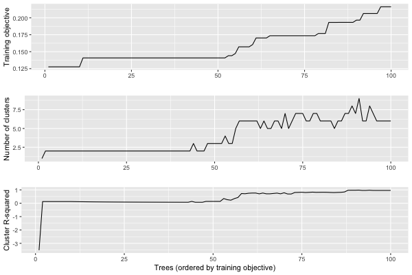
Stability Analysis
We conduct the stability analysis using stability_analysis:
stability <- iai::stability_analysis(lnr, train_X, train_y, criterion = "gini")
We can plot a summary of the analysis using plot.stability_analysis:
plot(stability)
We can use get_stability_results to extract the trees in order of training objective along with the importance of each feature in the tree:
iai::get_stability_results(stability)
   train_error tree_index  variance  skewness    curtosis entropy
1    0.1276390         38 0.6017131 0.3954914 0.002795447       0
2    0.1276773         21 0.6159242 0.2375321 0.146543689       0
3    0.1276773         22 0.6159242 0.2375321 0.146543689       0
4    0.1276773         29 0.6159242 0.2375321 0.146543689       0
5    0.1276773         39 0.6159242 0.2375321 0.146543689       0
6    0.1276773         55 0.6159242 0.2375321 0.146543689       0
7    0.1276773         59 0.6159242 0.2375321 0.146543689       0
8    0.1276773         70 0.6159242 0.2375321 0.146543689       0
9    0.1276773         96 0.6159242 0.2375321 0.146543689       0
10   0.1276773         97 0.6159242 0.2375321 0.146543689       0
 [ reached 'max' / getOption("max.print") -- omitted 90 rows ]
We can use get_cluster_details to summarize the clustering of the first 10 trees:
iai::get_cluster_details(stability, 10)
  train_error_mean  variance  skewness    curtosis entropy
1        0.1276390 0.6017131 0.3954914 0.002795447       0
2        0.1276773 0.6159242 0.2375321 0.146543689       0
We can use get_cluster_distances to get the relative distances between each pair of clusters:
iai::get_cluster_distances(stability, 10)
          [,1]      [,2]
[1,] 0.0000000 0.2140483
[2,] 0.2140483 0.0000000
We can use get_cluster_assignments to see which trees comprise each cluster:
iai::get_cluster_assignments(stability, 10)
[[1]]
[1] 38

[[2]]
[1] 21 22 29 39 55 59 70 96 97
We see that Tree 38 is in its own cluster, and the other trees are all grouped together. Given this, we might want to inspect how Tree 38 differs to the others. We can use get_tree to construct a new learner that uses the tree at a specified index:
iai::get_tree(lnr, 38)
We can also generate an interactive visualization that allows us to explore all of the information in the stability analysis using write_html or show_in_browser:
iai::write_html("stability_analysis.html", stability)
The resulting interactive visualization can be viewed here. As with all visualizations, this visualization is also automatically shown inside a Jupyter notebook.
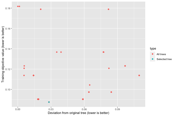
Similarity Comparison
We can also measure the stability of the training process to changes in the training data. We will use the following learner, trained on a variation of the training data:
We first use variable_importance_similarity to compute the difference between the original tree and each tree in the new learner, and feed this into similarity_comparison:
deviations <- iai::variable_importance_similarity(lnr, new_lnr, test_X, test_y,
                                                  criterion = "gini")
similarity <- iai::similarity_comparison(lnr, new_lnr, deviations)
We can plot a summary of the analysis using plot.similarity_comparison:
plot(similarity)
We can get the training objective values with get_train_errors:
train_errors <- iai::get_train_errors(similarity)
 [1] 0.12311935 0.09033247 0.09033247 0.09033247 0.09033247 0.09033247
 [7] 0.09033247 0.11373525 0.12311935 0.09734181 0.11373525 0.09033247
[13] 0.09033247 0.09033247 0.09033247 0.09033247 0.09033247 0.09033247
[19] 0.09033247 0.09033247 0.09033247 0.08750575 0.09734181 0.09734181
[25] 0.13668607 0.09033247 0.12074460 0.09033247 0.09033247 0.13668607
[31] 0.09033247 0.09734181 0.09033247 0.09033247 0.13668607 0.13668607
[37] 0.13668607 0.13668607 0.09033247 0.11373525 0.11373525 0.09033247
[43] 0.11373525 0.09033247 0.17885706 0.09033247 0.09033247 0.11373525
[49] 0.17885706 0.11373525 0.09033247 0.11373525 0.09033247 0.12311935
[55] 0.09033247 0.13668607 0.13668607 0.09033247 0.08750575 0.18168378
 [ reached getOption("max.print") -- omitted 40 entries ]
As we did for stability analysis, we can also generate an interactive visualization that allows us to explore all of the information in the similarity comparison using write_html or show_in_browser:
iai::write_html("similarity_comparison.html", similarity)
The resulting interactive visualization can be viewed here. As with all visualizations, this visualization is also automatically shown inside a Jupyter notebook.