Quick Start Guide: Heuristic Regressors
In this example we will use regressors from Heuristics on the yacht hydrodynamics dataset. First we load in the data and split into training and test datasets:
using CSV, DataFrames
df = DataFrame(CSV.File(
    "yacht_hydrodynamics.data",
    delim=' ',            # file uses ' ' as separators rather than ','
    ignorerepeated=true,  # sometimes columns are separated by more than one ' '
    header=[:position, :prismatic, :length_displacement, :beam_draught,
            :length_beam, :froude, :resistance],
))
308×7 DataFrame
Row │ position prismatic length_displacement beam_draught length_beam fr ⋯
│ Float64 Float64 Float64 Float64 Float64 Fl ⋯
─────┼──────────────────────────────────────────────────────────────────────────
1 │ -2.3 0.568 4.78 3.99 3.17 ⋯
2 │ -2.3 0.568 4.78 3.99 3.17
3 │ -2.3 0.568 4.78 3.99 3.17
4 │ -2.3 0.568 4.78 3.99 3.17
5 │ -2.3 0.568 4.78 3.99 3.17 ⋯
6 │ -2.3 0.568 4.78 3.99 3.17
7 │ -2.3 0.568 4.78 3.99 3.17
8 │ -2.3 0.568 4.78 3.99 3.17
⋮ │ ⋮ ⋮ ⋮ ⋮ ⋮ ⋱
302 │ -2.3 0.6 4.34 4.23 2.73 ⋯
303 │ -2.3 0.6 4.34 4.23 2.73
304 │ -2.3 0.6 4.34 4.23 2.73
305 │ -2.3 0.6 4.34 4.23 2.73
306 │ -2.3 0.6 4.34 4.23 2.73 ⋯
307 │ -2.3 0.6 4.34 4.23 2.73
308 │ -2.3 0.6 4.34 4.23 2.73
2 columns and 293 rows omittedX = df[:, 1:(end - 1)]
y = df[:, end]
(train_X, train_y), (test_X, test_y) = IAI.split_data(:regression, X, y, seed=1)Random Forest Regressor
We will use a GridSearch to fit a RandomForestRegressor with some basic parameter validation:
grid = IAI.GridSearch(
    IAI.RandomForestRegressor(
        random_seed=1,
    ),
    max_depth=5:10,
)
IAI.fit!(grid, train_X, train_y)
All Grid Results:
Row │ max_depth train_score valid_score rank_valid_score
│ Int64 Float64 Float64 Int64
─────┼───────────────────────────────────────────────────────
1 │ 5 0.994449 0.990294 6
2 │ 6 0.994511 0.990322 1
3 │ 7 0.994515 0.990321 2
4 │ 8 0.994515 0.990321 3
5 │ 9 0.994515 0.990321 4
6 │ 10 0.994515 0.990321 5
Best Params:
max_depth => 6
Best Model - Fitted RandomForestRegressorWe can make predictions on new data using predict:
IAI.predict(grid, test_X)92-element Vector{Float64}:
0.12836191255
0.24591597504
1.293050230222
2.854614345067
5.201156146354
13.586306926407
20.989118226218
0.12756191255
0.24591597504
0.497498593494
⋮
2.872119106971
8.033722622378
13.586306926407
1.280463765576
1.979024639249
2.896419464114
13.862548174881
33.505260589966
53.294637063492We can evaluate the quality of the model using score with any of the supported loss functions. For example, the $R^2$ on the training set:
IAI.score(grid, train_X, train_y, criterion=:mse)0.9954616758740213Or on the test set:
IAI.score(grid, test_X, test_y, criterion=:mse)0.9898501909798273We can also look at the variable importance:
IAI.variable_importance(IAI.get_learner(grid))6×2 DataFrame
Row │ Feature Importance
│ Symbol Float64
─────┼──────────────────────────────────
1 │ froude 0.994405
2 │ prismatic 0.00165704
3 │ length_displacement 0.00161713
4 │ beam_draught 0.00142863
5 │ length_beam 0.000663934
6 │ position 0.000227865XGBoost Regressor
We will use a GridSearch to fit a XGBoostRegressor with some basic parameter validation:
grid = IAI.GridSearch(
    IAI.XGBoostRegressor(
        random_seed=1,
    ),
    max_depth=2:5,
    num_round=[20, 50, 100],
)
IAI.fit!(grid, train_X, train_y)
All Grid Results:
Row │ num_round max_depth train_score valid_score rank_valid_score
│ Int64 Int64 Float64 Float64 Int64
─────┼──────────────────────────────────────────────────────────────────
1 │ 20 2 0.99756 0.993216 3
2 │ 20 3 0.999231 0.99266 9
3 │ 20 4 0.999735 0.993189 4
4 │ 20 5 0.999831 0.99201 10
5 │ 50 2 0.999287 0.995097 2
6 │ 50 3 0.999892 0.993184 5
7 │ 50 4 0.999959 0.992946 7
8 │ 50 5 0.999973 0.990473 11
9 │ 100 2 0.999698 0.996021 1
10 │ 100 3 0.9999 0.993153 6
11 │ 100 4 0.999959 0.992946 8
12 │ 100 5 0.999973 0.990472 12
Best Params:
num_round => 100
max_depth => 2
Best Model - Fitted XGBoostRegressorWe can make predictions on new data using predict:
IAI.predict(grid, test_X)92-element Vector{Float64}:
0.23346585
0.37805766
1.26587629
2.81103897
5.41519117
12.59898853
20.52502441
0.21097377
0.25714141
0.42428526
⋮
2.81908727
7.73881865
12.53344631
1.45720315
2.09043741
3.00236559
11.98634815
33.26702881
49.76499939We can evaluate the quality of the model using score with any of the supported loss functions. For example, the $R^2$ on the training set:
IAI.score(grid, train_X, train_y, criterion=:mse)0.99950684Or on the test set:
IAI.score(grid, test_X, test_y, criterion=:mse)0.99734513We can also look at the variable importance:
IAI.variable_importance(IAI.get_learner(grid))6×2 DataFrame
Row │ Feature Importance
│ Symbol Float64
─────┼─────────────────────────────────
1 │ froude 0.954647
2 │ length_displacement 0.0182929
3 │ prismatic 0.0139216
4 │ beam_draught 0.00639543
5 │ position 0.00411147
6 │ length_beam 0.00263133We can calculate the SHAP values:
s = IAI.predict_shap(grid, test_X)
s[:shap_values]
92×6 Matrix{Float64}:
-0.0632808 -0.0114608 -0.0391644 -0.0184659 -0.0815269 -9.86757
-0.0664552 -0.0114608 -0.0378506 -0.0076839 -0.0815269 -9.7319
-0.0723957 -0.012742 -0.0430042 0.00760984 -0.134582 -8.79394
-0.0723957 -0.00525591 -0.0430042 0.0375999 -0.134582 -7.28626
-0.175767 0.000270572 -0.0390034 0.0418154 -0.17572 -4.55134
-0.214559 -0.196073 -0.0348593 0.000398656 -0.160192 2.88934
-0.205349 -0.493743 -0.0348593 -0.0975699 -0.204386 11.246
-0.0632808 -0.0534274 -0.0380514 0.0455295 0.026066 -10.0208
-0.0664552 -0.0534274 -0.0367376 0.0070994 0.026066 -9.93434
-0.0723957 -0.0534274 -0.0367376 0.0070994 0.00867438 -9.74386
⋮ ⋮
-0.0767186 -0.128861 0.00186686 0.0375999 -0.11716 -7.21257
-0.18009 -0.177774 0.00586762 0.0418154 -0.158297 -2.10764
-0.218882 -0.342035 -0.00442569 0.000398656 -0.142769 2.92623
-0.0809773 -0.140015 0.0713933 0.00760984 0.13303 -8.84877
-0.0809773 -0.138004 0.0713933 0.0184519 0.13303 -8.22839
-0.0809773 -0.132529 0.0713933 0.0375999 0.13303 -7.34109
-0.223141 -0.345702 0.0795381 0.000398656 -0.272206 2.43253
-0.147518 -0.643373 0.5539 -0.30065 -0.273265 23.763
-0.17315 -1.51305 0.799156 -0.285291 0.132692 40.4897We can then use the SHAP library in Python to visualize these results in whichever way we prefer. For example, the following code creates a summary plot:
using PyCall
shap = pyimport("shap")
shap.summary_plot(s[:shap_values], Matrix(s[:features]), names(s[:features]))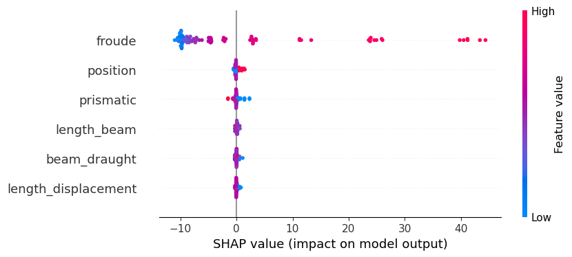
GLMNet Regressor
We can use a GLMNetCVRegressor to fit a GLMNet model using cross-validation:
lnr = IAI.GLMNetCVRegressor(
    random_seed=1,
    n_folds=10,
)
IAI.fit!(lnr, train_X, train_y)
Fitted GLMNetCVRegressor:
Constant: -22.2638
Weights:
froude: 113.914We can access the coefficients from the fitted model with get_prediction_weights and get_prediction_constant:
numeric_weights, categoric_weights = IAI.get_prediction_weights(lnr)
numeric_weights
Dict{Symbol, Float64} with 1 entry:
:froude => 113.914categoric_weightsDict{Symbol, Dict{Any, Float64}}()IAI.get_prediction_constant(lnr)-22.263799We can make predictions on new data using predict:
IAI.predict(lnr, test_X)92-element Vector{Float64}:
-8.024522
-5.176667
3.366899
9.06261
14.758321
20.454031
23.301887
-8.024522
-5.176667
-2.328811
⋮
9.06261
17.606176
20.454031
3.366899
6.214755
9.06261
20.454031
26.149742
28.997597We can evaluate the quality of the model using score with any of the supported loss functions. For example, the $R^2$ on the training set:
IAI.score(lnr, train_X, train_y, criterion=:mse)0.654571718994Or on the test set:
IAI.score(lnr, test_X, test_y, criterion=:mse)0.651006827713We can also look at the variable importance:
IAI.variable_importance(lnr)6×2 DataFrame
Row │ Feature Importance
│ Symbol Float64
─────┼─────────────────────────────────
1 │ froude 1.0
2 │ beam_draught 0.0
3 │ length_beam 0.0
4 │ length_displacement 0.0
5 │ position 0.0
6 │ prismatic 0.0