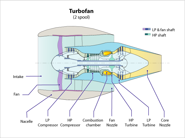
Turbofan: an interpretable predictive maintenance case
Predictive maintenance aims to find the right moment to perform maintenance so that an industrial system's components are not prematurely replaced while ensuring the reliability of the whole system. As complexity of industrial systems grows, understanding the ways in which they can fail becomes all the more challenging.
In this case study, we build models to help quantify the risk of failure for a machine in any moment and we illustrate how interpretability helps to understand the underlying failure mechanisms through two approaches:
- Predict failure within a given time window. We compare how Optimal Classification Trees compare to CART and XGBoost with respect to interpretability and performance.
- Predict the probability of failure over time with our novel Optimal Survival Tree algorithm.
We conduct our analysis on the turbofan dataset, released by NASA to study engine degradation.
Turbofan Datasets
The turbofan datasets present the following characteristics:
- Each dataset consists of multiple multivariate time series, generated by a physical model of the turbofan.
- Each dataset simulates the behavior of a turbofan in different atmospheric conditions and with different fault modes.
- Each time series is from a different engine, i.e., the data can be considered to be from a fleet of engines of the same type.
- Each engine starts with different degrees of initial wear and manufacturing variation which is unknown to the user. This wear and variation is considered normal, i.e., it is not considered a fault condition.
- There are three operational settings that have a substantial effect on engine performance. These settings are also included in the data.
- The engine is operating normally at the start of each time series, and develops a fault at some point during the series.
- The data is contaminated with sensor noise.
Data Reading
We load the dataset 'FD_003':
- It records 20k+ daily observations for 100 failure trajectories
- Each engine is evaluated in the same atmospheric conditions
- There are two causes of failure: High Pressure Compressor (HPC) degradation and fan degradation
import pandas as pd
name_df = pd.DataFrame(
    columns=['sensor_id', 'sensor_name', 'sensor_description'],
    data=[
        ['sensor_01', 'T2', 'Total temperature at fan inlet'],
        ['sensor_02', 'T24', 'Total temperature at LPC outlet'],
        ['sensor_03', 'T30', 'Total temperature at HPC outlet'],
        ['sensor_04', 'T50', 'Total temperature at LPT outlet'],
        ['sensor_05', 'P2', 'Pressure at fan inlet'],
        ['sensor_06', 'P15', 'Total pressure in bypass-duct'],
        ['sensor_07', 'P30', 'Total pressure at HPC outlet'],
        ['sensor_08', 'Nf', 'Physical fan speed'],
        ['sensor_09', 'Nc', 'Physical core speed'],
        ['sensor_10', 'epr', 'Engine pressure ratio (P50/P2)'],
        ['sensor_11', 'Ps30', 'Static pressure at HPC outlet'],
        ['sensor_12', 'phi', 'Ratio of fuel flow to Ps30'],
        ['sensor_13', 'NRf', 'Corrected fan speed'],
        ['sensor_14', 'NRc', 'Corrected core speed'],
        ['sensor_15', 'BPR', 'Bypass Ratio'],
        ['sensor_16', 'farB', 'Burner fuel-air ratio'],
        ['sensor_17', 'htBleed', 'Bleed Enthalpy'],
        ['sensor_18', 'Nf_dmd', 'Demanded fan speed'],
        ['sensor_19', 'PCNfR_dmd', 'Demanded corrected fan speed'],
        ['sensor_20', 'W31', 'HPT coolant bleed'],
        ['sensor_21', 'W32', 'LPT coolant bleed'],
        ['sensor_22', 'T48', 'Total temperature at HPT outlet'],
        ['sensor_23', 'SmFan', 'Fan stall margin'],
        ['sensor_24', 'SmLPC', 'LPC stall margin'],
        ['sensor_25', 'SmHPC', 'HPC stall margin'],
    ],
)
name_df.set_index('sensor_id', inplace=True)

names = ['unit_nr', 'time', 'operation_setting_1', 'operation_setting_2',
         'condition_3']
names += name_df.sensor_name.to_list()

df = pd.read_csv('train_FD003.txt', sep=' ', header=None, names=names,
                 index_col=False)
Data Cleaning
We remove columns with no values or with only one value
df.dropna(how='all', axis=1, inplace=True)
cols_const = [col for col in df.columns if len(df[col].unique()) <= 2]
df.drop(columns=cols_const, inplace=True)
       unit_nr  time  operation_setting_1  ...  htBleed    W31      W32
0            1     1              -0.0005  ...      391  39.11  23.3537
1            1     2               0.0008  ...      392  38.99  23.4491
2            1     3              -0.0014  ...      391  38.85  23.3669
3            1     4              -0.0020  ...      392  38.96  23.2951
4            1     5               0.0016  ...      392  39.14  23.4583
5            1     6               0.0011  ...      393  38.92  23.4281
6            1     7              -0.0038  ...      391  38.84  23.4087
...        ...   ...                  ...  ...      ...    ...      ...
24713      100   146               0.0016  ...      396  38.41  23.1246
24714      100   147               0.0004  ...      395  38.59  23.0528
24715      100   148              -0.0016  ...      394  38.44  22.9631
24716      100   149               0.0034  ...      395  38.50  22.9746
24717      100   150              -0.0016  ...      396  38.39  23.0682
24718      100   151              -0.0023  ...      395  38.31  23.0753
24719      100   152               0.0000  ...      396  38.56  23.0847

[24720 rows x 20 columns]
Add remaining useful life (RUL) column
For each unit, we compute the time remaining before the engine failure occured.
mapper = {}
for unit_nr in df['unit_nr'].unique():
    mapper[unit_nr] = df['time'].loc[df['unit_nr'] == unit_nr].max()

df['RUL'] = df['unit_nr'].apply(lambda nr: mapper[nr]) - df['time'] + 1
Data Visualization
We can plot the signals measured by the 18 sensors (Y-axis) over time (X-axis) for a given machine.
import matplotlib.pyplot as plt
df_unit = df[df.unit_nr == 1]
fig = plt.figure(figsize=(20, 25))
for i, col in enumerate(df_unit.columns[2:-1]):
    ax = fig.add_subplot(6, 3, i+1)
    df_unit.plot.scatter('time', col, title=col, ax=ax)
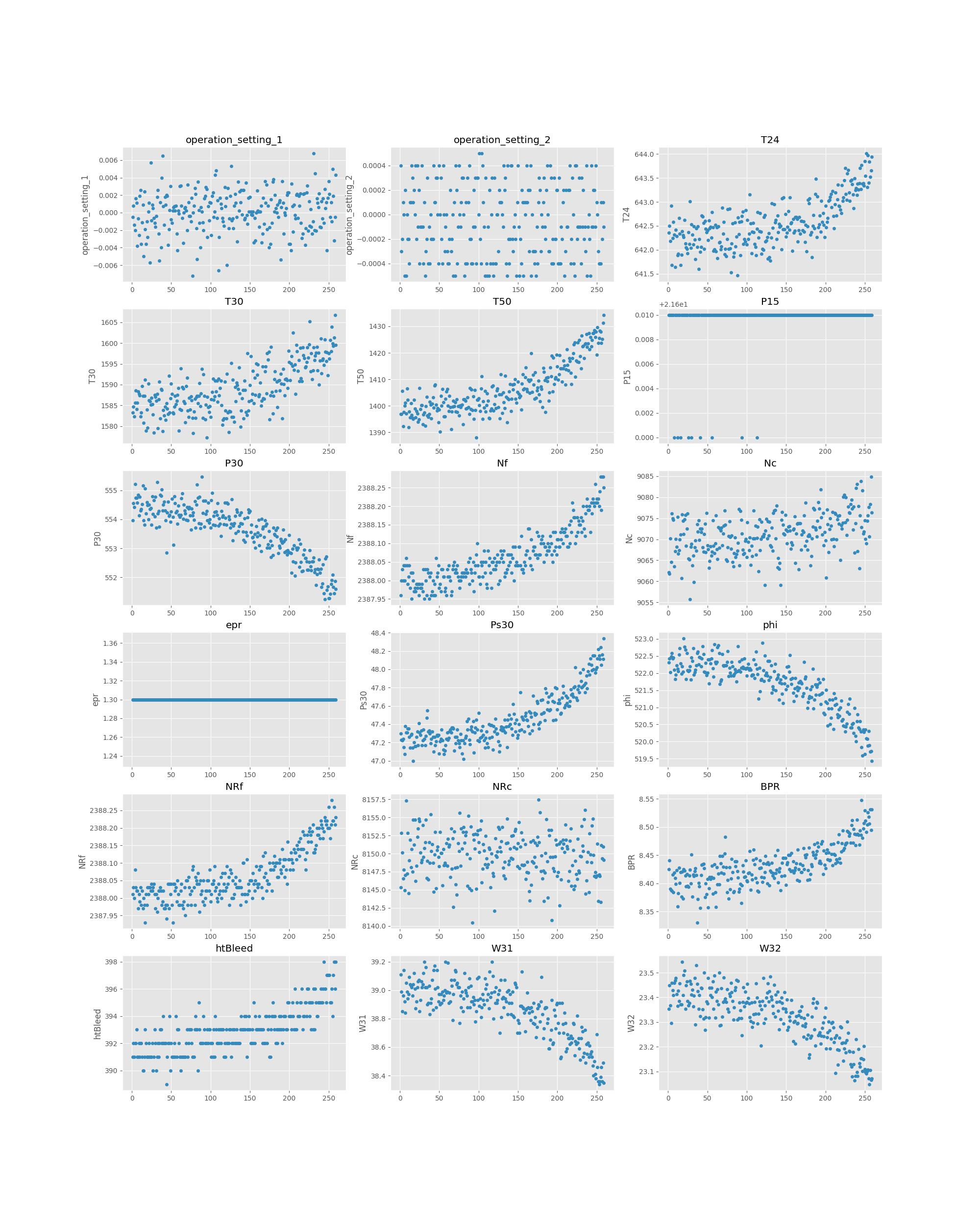
We observe that as the engine gets used, most sensors record a monotonous trend (not accounting for noise). This illustrates the fact that all the modules of the turbofan are influencing each other's behavior and lifetime. The goal of analysis will be to understand what behaviors forewarn failures and how the faults propagate through the entire system.
Predict Next Day Failures
We transform our predictive maintenance problem to a classification task. Our goal here is to predict whether the machine will fail on the following day, given the measurements available up to that day.
Data Preprocessing
In real-life scenarios, it may be rare to have this many data points. We keep 1500 normal measurements and 100 failures to reduce the number of observed measurements while keeping the class imbalance.
df_error = df[df.RUL == 2].reset_index(drop=True)
df_no_error = df[df.RUL > 2].reset_index(drop=True)
df_no_error = df_no_error.sample(n=1500, random_state=0).reset_index(drop=True)

df_sampled = pd.concat([df_error, df_no_error]).reset_index(drop=True)
df_sampled = df_sampled.sample(frac=1, random_state=0).reset_index(drop=True)
df_sampled['error'] = df_sampled['RUL'] == 2

df_class = df_sampled.drop(columns=['unit_nr', 'time', 'RUL'])
We randomly split our data into training and testing. All models will be trained on the same training set and evaluated on the same testing set.
from interpretableai import iai
X = df_class.iloc[:, :-1]
y = df_class.iloc[:, -1]
(train_X, train_y), (test_X, test_y) = iai.split_data('classification', X, y,
                                                      seed=1)
CART
We first run the classical Classification and Regression Tree (CART) method. Given how understandable decision trees are, CART is often the first method considered when interpretability matters.
grid = iai.GridSearch(
    iai.OptimalTreeClassifier(
        random_seed=1,
        localsearch=False,
        missingdatamode='separate_class',
        criterion='gini',
    ),
    max_depth=range(1, 10),
)
grid.fit(train_X, train_y)
grid.get_learner()
train_auc = grid.score(train_X, train_y, criterion='auc')
test_auc = grid.score(test_X, test_y, criterion='auc')
{'train_auc': train_auc, 'test_auc': test_auc}
{'train_auc': 0.9885646258503401, 'test_auc': 0.9070740740740743}The AUC on the training set is high but despite the validation on the depth and complexity parameter, the lower AUC in testing indicates that the model overfits to the data.
Consequently, we have to be careful, because despite the interpretability of the model, the relationships found may be mere artifacts of the training data and its noise. This model is therefore not reliable to understand the interactions between the system's components and false positives are likely to be predicted.
XGBoost
We then run XGBoost, which is a good way to quickly achieve very strong performance in predictive tasks.
xgb = iai.XGBoostClassifier()
xgb.fit(train_X, train_y)

train_auc = xgb.score(train_X, train_y, criterion='auc')
test_auc = xgb.score(test_X, test_y, criterion='auc')
{'train_auc': train_auc, 'test_auc': test_auc}
{'train_auc': 0.999999999999994, 'test_auc': 0.9923703703703715}The results are excellent in term of AUC, but there is little information available to understand the logic underlying the decisions the algorithm makes. We can try to use a method like SHAP to understand how the model uses the features. First, we calculate the SHAP values:
s = xgb.predict_shap(test_X)
We can then use the SHAP library to visualize these values. For instance, we can summarize the importance of every feature in the model:
import shap
shap.summary_plot(s['shap_values'][1], s['features'])
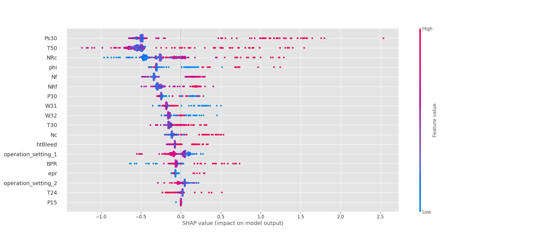
This gives us some idea as to which features are important in the model, but it is difficult to understand further than this.
For more details on how to explain XGBoost models and how they compare with the interpretability of Optimal Trees, please refer to the Loan Default Risk case study.
Optimal Trees
grid = iai.GridSearch(
    iai.OptimalTreeClassifier(
        random_seed=1,
        missingdatamode='separate_class',
        criterion='gini',
    ),
    max_depth=range(2, 4),
)
grid.fit_cv(train_X, train_y)
grid.get_learner()
train_auc = grid.score(train_X, train_y, criterion='auc')
test_auc = grid.score(test_X, test_y, criterion='auc')
{'train_auc': train_auc, 'test_auc': test_auc}
{'train_auc': 0.9956530612244897, 'test_auc': 0.9526296296296296}We make the following observations about the Optimal Classification Tree (OCT) model:
The performance is significantly better out-of sample than CART and closer to that of the XGBoost model. This gives us a lot more confidence that the splits in the tree are reflecting the true relationships in the data rather than noise.
A small number of features are picked up by the model to predict failures. The model is therefore simple enough to understand the logic behind the predictions it makes. For instance in our case, it allows engine experts to link the decisions the tree makes to underlying physical processes:
- If the physical core speed (
Nc) is high, this increases the likelihood of failure. In this case, either the combination of a low HTP coolant bleed (W31) and low fuel flow (phi) or a high HTP coolant bleed and high pressure at the high pressure compressor (Ps30) are indicative of failure. - If the physical core speed is low, the risk of failure depends on interactions between the core speed (
NRc) and fan speed (NRfandNf).
- If the physical core speed (
The features picked up by the model are also among the most important features in the XGBoost model.
The tree gives both a good prediction of failure events but also allows experts to understand the underlying mechanisms that lead to failures. These insights can also motivate further actions such as designing ways to maintain a low pressure in the HPC in case of failure so that it does not affect the entire system.
Predict Survival Time Distribution
Previously our models have predicted whether the machine is going to fail on a given day, but we can also predict the distribution of time before failure with our Optimal Survival Tree module. In this model, each node of the tree contains a survival curve that describes how the failure rate varies with time across observations in that node.
This type of analysis allows to answer the following questions:
- What is the likelihood of a turbofan functioning past a certain time?
- Of those that survive, at what rate will they fail?
- How do particular circumstances or characteristics increase or decrease the probability of survival?
The survival function denoted $S$ is defined as $S(t)=\mathcal{P}(T>t)$ where $t$ is some time and $T$ is a random variable denoting the time of failure.
In our case, survival analysis focuses on the expected duration of time until occurrence of a failure. However, the event may not be observed for some machines within the study time period, producing so-called censored observations. Censoring may arise in the following ways:
- a turbofan has not yet experienced a failure within the study time period
- a turbofan ceases to be used before failure
- a turbofan is repaired before failure is observed
This type of censoring, named right censoring, is handled in survival analysis. For more information on the data format, refer to the data preparation guide.
First, we prepare the data and split into training and testing:
import numpy as np
X = df.drop(columns=['RUL','time', 'unit_nr'])
failure = pd.Series(np.ones(df.shape[0])).astype(bool)
times = df.RUL

(train_X, train_failure, train_times), (test_X, test_failure, test_times) = \
    iai.split_data('survival', X, failure, times, seed=1)
Next, we can train the Optimal Survival Tree:
grid = iai.GridSearch(
    iai.OptimalTreeSurvivalLearner(
        random_seed=1,
        missingdatamode='separate_class',
    ),
    max_depth=range(2, 3),
)
grid.fit(train_X, train_failure, train_times,
         validation_criterion='harrell_c_statistic')
grid.get_learner()
We can evaluate the quality of our model using the Harrell C-statistic. It is analogous to the AUC and ranges from 0.5 (minimum score) to 1 (maximum score).
train_harrell_score = grid.score(train_X, train_failure, train_times,
                                 criterion='harrell_c_statistic')
test_harrell_score = grid.score(test_X, test_failure, test_times,
                                criterion='harrell_c_statistic')
{'train_harrell_score': train_harrell_score,
 'test_harrell_score': test_harrell_score}
{'train_harrell_score': 0.7574595865587105, 'test_harrell_score': 0.7571946087159976}In this case, the tree uses the outlet pressure of the HPC module (Ps30) and the physical core speed (Nc). Previously, we showed that these features (or derivatives) were key in the detection of failures, since they were affected when either the HPC or the fan were at fault.