Coordinated-Sparsity Fitting

There are times when it is desirable to fit linear models to multiple linked datasets. Examples include:

clustering a dataset and then fitting linear/logistic regression models in each of the resulting clusters
fitting linear/logistic regression models in each leaf of a decision tree

If we are seeking sparse models in each of these clusters, we might choose to fit the models with Optimal Feature Selection to restrict their sparsity. However, this may not necessarily result in a sparse selection of features from the overall dataset, because even though each model is restricted in the number of features it can choose, each of the models can choose an entirely different set of features. As a concrete example, if we have 10 clusters and restrict the sparsity to 5, we might still end up with as many as 50 features selected.

Bertsimas et al. (2021) address this problem by introducing a method for fitting multiple regression models with a coordinated sparsity restriction. This approach constrains the models in each cluster to use the same set of features, and optimizes this set of features to find the best overall fit for the data. In the example from above, it will find the set of 5 features to use across all of the 10 clusters that results in the best overall fit.

On this page, we demonstrate how to apply this coordinated-sparsity algorithm on a synthetic regression problem, but the same approach also applies to classification problems.

Manual Clustering

First, we will demonstrate how to use the coordinated-sparsity approach on data with pre-defined clusters. We will generate random features:

using StableRNGs, DataFrames
rng = StableRNG(1) # for consistent output across Julia versions
n = 500
p = 10
X = DataFrame(rand(rng, n, p), :auto)

Our target will be the following simple piecewise-linear function:

\[y = \begin{cases} x_2 + 3 x_3, & \text{if } x_1 < 0.5\\ 0.5x_2 + x_4, & \text{otherwise} \end{cases}\]

We will generate our target data according to this function with the addition of a small amount of noise:

y = ((X.x1 .< 0.5) .* (X.x2 .+ 3 .* X.x3)) .+
    ((X.x1 .> 0.5) .* (0.5 .* X.x2 .- X.x4)) .+
    0.1 .* randn(rng, n)

We know from the data generation process that there are two clusters in the data, but we can also attempt to identify this ourselves from the data. To do this, we try fitting a simple linear model to the entire dataset:

lnr = IAI.OptimalFeatureSelectionRegressor(random_seed=1, sparsity=3)
IAI.fit!(lnr, X, y)

Fitted OptimalFeatureSelectionRegressor:
  Constant: 2.07097
  Weights:
    x1: -3.17664
    x3:  1.51278
    x4: -0.64826

We see that $x_1$ seems important, and so we can plot the relationship between this feature and the target to investigate further:

using Plots
scatter(X.x1, y)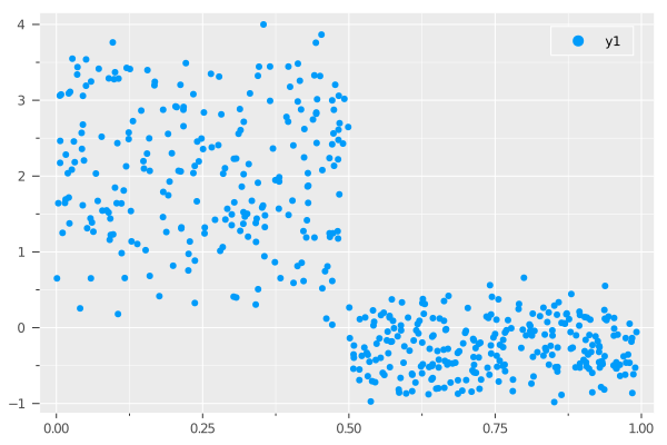

We can indeed clearly see the two clusters in the data, separated by the line $x_1 = 0.5$. Using this, we can extract the set of indices in our dataset that fall into each cluster:

cluster_inds = [findall(X.x1 .< 0.5), findall(X.x1 .> 0.5)]

2-element Vector{Vector{Int64}}:
 [2, 4, 6, 9, 10, 12, 14, 15, 16, 18  …  481, 484, 485, 487, 488, 489, 490, 492, 493, 500]
 [1, 3, 5, 7, 8, 11, 13, 17, 19, 21  …  482, 483, 486, 491, 494, 495, 496, 497, 498, 499]

We can now conduct the coordinated-sparsity fitting. To do this, we use a normal OptimalFeatureSelectionRegressor and set coordinated_sparsity=true in addition to any other parameters. Then, when fitting the model, we pass the indices of points that fall into each of the clusters, and the algorithm will fit models in each of these clusters with the constraint that the features used across all clusters are the same:

lnr = IAI.OptimalFeatureSelectionRegressor(random_seed=1, sparsity=3,
                                           coordinated_sparsity=true)
IAI.fit!(lnr, X, y, cluster_inds=cluster_inds)

Fitted OptimalFeatureSelectionRegressor:
  Model for cluster 1:
    Constant: 0.120663
    Weights:
      x2:  0.954967
      x3:  2.79626
      x4:  0.0158888

  Model for cluster 2:
    Constant: -0.0175999
    Weights:
      x2:  0.471342
      x3: -0.0199532
      x4: -0.93334

We see that indeed the models in each cluster use the same set of features.

We can access the model coefficients using the get_prediction_weights and get_prediction_constant functions as normal, with the addition of the fit_index keyword argument to specify which cluster we are querying:

IAI.get_prediction_constant(lnr, fit_index=1)

0.1206627455

IAI.get_prediction_constant(lnr, fit_index=2)

-0.0175998969

Similarly, we can use the score and predict functions with fit_index as a keyword argument to evaluate performance or make predictions for the model in a given cluster:

IAI.predict(lnr, X, fit_index=1)

500-element Vector{Float64}:
 3.0278138976
 2.6674048668
 2.2530380577
 2.5102592056
 2.3218138264
 0.4636159461
 2.1997303223
 1.2857690034
 3.1790294205
 1.0155637819
 ⋮
 1.1163276932
 1.2153502241
 1.4717940265
 0.8039731273
 1.8097329494
 2.9856877131
 1.626650041
 2.4573154806
 1.1980484587

Integration with Optimal Trees

Another use-case for coordinated-sparsity fitting is in conjunction with trained tree models. We often want to fit linear models in the leaves of the tree, and further it can be desirable for these models to be sparse. The coordinated-sparsity approach can help with controlling the total number of features used across all of the leaves in the tree.

As this example is a regression problem, we can train directly with linear models in the leaves by setting regression_sparsity=:all :

grid = IAI.GridSearch(
    IAI.OptimalTreeRegressor(random_seed=1, regression_features=All()),
    max_depth=1,
)
IAI.fit!(grid, X, y)
lnr = IAI.get_learner(grid)

Optimal Trees Visualization

While we obtain a tree with linear regression models in each leaf, we see that these models use a lot of features, and we might prefer if these models were sparser. One option to reduce the number of features selected is to use refit_leaves! with an OptimalFeatureSelectionRegressor as the refit_learner to refit the leaves of the tree with sparse regression models:

refit_learner = IAI.OptimalFeatureSelectionRegressor(random_seed=1, sparsity=3)
IAI.refit_leaves!(lnr, X, y, refit_learner=refit_learner)

Optimal Trees Visualization

We see the sparsity is reduced from before, but even though each leaf was constrained to use just three features, we have still used a total of five features across the two leaves. We might want to know if this total could be reduced further by using the same features in each leaf, but since each leaf is refit independently, this uncoordinated approach has little control over the total number of features used across the entire model.

To rectify this and gain control over the total number of features used across all the models, we can set coordinated_sparsity=true on the refit_learner, which will use coordinated-sparsity fitting to find the best set of features that work well across all leaves:

refit_learner.coordinated_sparsity = true
IAI.refit_leaves!(lnr, X, y, refit_learner=refit_learner)

Optimal Trees Visualization

We see that now the model in each leaf uses the same three features, which is a reduction from the five features selected without the coordinated-sparsity restriction.

We can also embed the coordinated-sparsity refit in the tree training process by setting refit_learner on the tree learner directly:

grid = IAI.GridSearch(
    IAI.OptimalTreeRegressor(random_seed=1, refit_learner=refit_learner),
    max_depth=1,
)
IAI.fit!(grid, X, y)
lnr = IAI.get_learner(grid)

Optimal Trees Visualization

In this case, we arrive at the same solution as approach using refit_leaves!, but in other applications this may not be the case, so it may be worth considering both approaches.

Coordinated-sparsity refitting can also be used for classification trees by using OptimalFeatureSelectionClassifier with coordinated_sparsity=true as the refit_learner in any of the approaches detailed in the documentation for fitting logistic regression in the leaves.