Predicting House Sale Prices

In this example, we aim to predict the sales price of houses in King County, Washington, using a dataset available on Kaggle. We will start with Optimal Regression Trees with constant predictions. The results give us evidence to suspect that there are strong linear effects that could be modeled more directly. We use Optimal Sparse Regression to detect the key linear predictor, and fit Optimal Regression Trees with linear predictions using this variable. We show this careful modeling leads to significant gains in both performance and interpretability.

Data Preparation

First, we load the data and create the features and labels:

using CSV, DataFrames
data = CSV.read("kc_house_data.csv", DataFrame)

using CategoricalArrays
categoric = [
    :waterfront,
]
ordinal = [
    :condition,
    :view,
    :grade,
]
continuous = [
    :floors,
    :bedrooms,
    :bathrooms,
    :sqft_above,
    :sqft_basement,
    :yr_built,
    :yr_renovated,
    :sqft_living,
    :sqft_lot,
    :lat,
    :long,
    :sqft_living15,
    :sqft_lot15,
]
X = select(data,
    categoric .=> categorical,
    ordinal .=> c -> categorical(c, ordered=true),
    continuous,
    renamecols=false,
)

y = data.price

X

21613×17 DataFrame
   Row │ waterfront  condition  view  grade  floors   bedrooms  bathrooms  sqf ⋯
       │ Cat…        Cat…       Cat…  Cat…   Float64  Int64     Float64    Int ⋯
───────┼────────────────────────────────────────────────────────────────────────
     1 │ 0           3          0     7          1.0         3       1.0       ⋯
     2 │ 0           3          0     7          2.0         3       2.25
     3 │ 0           3          0     6          1.0         2       1.0
     4 │ 0           5          0     7          1.0         4       3.0
     5 │ 0           3          0     8          1.0         3       2.0       ⋯
     6 │ 0           3          0     11         1.0         4       4.5
     7 │ 0           3          0     7          2.0         3       2.25
     8 │ 0           3          0     7          1.0         3       1.5
   ⋮   │     ⋮           ⋮       ⋮      ⋮       ⋮        ⋮          ⋮          ⋱
 21607 │ 0           3          0     9          2.0         4       3.5       ⋯
 21608 │ 0           3          0     8          2.0         3       2.5
 21609 │ 0           3          0     8          3.0         3       2.5
 21610 │ 0           3          0     8          2.0         4       2.5
 21611 │ 0           3          0     7          2.0         2       0.75      ⋯
 21612 │ 0           3          0     8          2.0         3       2.5
 21613 │ 0           3          0     7          2.0         2       0.75
                                               10 columns and 21598 rows omitted

We split the data into training and testing:

seed = 123
(X_train, y_train), (X_test, y_test) =
    IAI.split_data(:regression, X, y, seed=seed, train_proportion=0.5)

Regression Tree with Constant Predictions

First, we will try a simple regression tree with constant predictions to gain some understanding of the various features interact:

grid_constant_tree = IAI.GridSearch(
    IAI.OptimalTreeRegressor(random_seed=seed, minbucket=50),
    max_depth=1:5,
)
IAI.fit!(grid_constant_tree, X_train, y_train)

Optimal Trees Visualization

We observe a lot of times that sqft_living (square footage of the apartments interior living space) is used in splitting. It is not surprising that this variable is important in predicting sales price. In fact, human intuition would tell us that there is likely a strong linear relationship between the living space and the sales price.

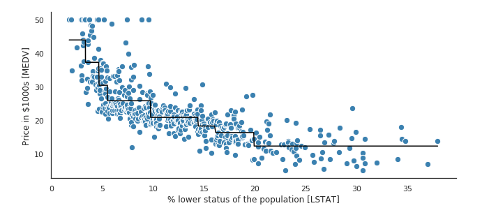
Unfortunately, traditional trees with constant predictions in each leaf are not good at learning linear effects. As can be seen in the example below, the predictions from the tree form a piecewise-constant function, and we need many splits to accurately approximate a linear function.

Detecting Linear Effects

To test if there is indeed a strong linear relationship, we can try a sparse regression:

grid_sparse_regression = IAI.GridSearch(
    IAI.OptimalFeatureSelectionRegressor(random_seed=seed),
    sparsity=1:5,
)
IAI.fit!(grid_sparse_regression, X_train, y_train)

All Grid Results:

 Row │ sparsity  train_score  valid_score  rank_valid_score
     │ Int64     Float64      Float64      Int64
─────┼──────────────────────────────────────────────────────
   1 │        1     0.506632     0.462836                 5
   2 │        2     0.571826     0.555002                 4
   3 │        3     0.614329     0.584549                 3
   4 │        4     0.646008     0.628425                 1
   5 │        5     0.663746     0.624787                 2

Best Params:
  sparsity => 4

Best Model - Fitted OptimalFeatureSelectionRegressor:
  Constant: -32532188.2
  Weights:
    grade≤10:    -534130.2
    lat:          700525.2
    sqft_living:  224.772
    view=0:      -209369

We see that the model did pick up a number of linear predictors, including sqft_living as we had expected. However, since the variables have very different scales we cannot simply interpret these coefficients to understand the importance of each feature. Instead, we can examine the importance of each feature:

IAI.variable_importance(IAI.get_learner(grid_sparse_regression))

49×2 DataFrame
 Row │ Feature       Importance
     │ Symbol        Float64
─────┼──────────────────────────
   1 │ sqft_living     0.462803
   2 │ lat             0.219461
   3 │ grade≤10        0.17567
   4 │ view=0          0.142066
   5 │ bathrooms       0.0
   6 │ bedrooms        0.0
   7 │ condition=1     0.0
   8 │ condition=2     0.0
  ⋮  │      ⋮            ⋮
  43 │ view=3          0.0
  44 │ view=4          0.0
  45 │ view≤1          0.0
  46 │ view≤2          0.0
  47 │ waterfront=1    0.0
  48 │ yr_built        0.0
  49 │ yr_renovated    0.0
                 34 rows omitted

We see that sqft_living is in fact the most important variables in terms of effect on the sales price.

Regression Tree with Linear Predictions

A major drawback of the linear model is that it assigns the same weight on sqft_living to houses of very different natures, which may not be the case in reality. For instance, we might expect houses in better locations to have a higher marginal benefit from additional living space. This is a scenario where a regression tree with linear predictions is well-suited: it models a piecewise-linear relationship. Let's try fitting an Optimal Regression Tree with sqft_living as the linear regressor:

grid_regression_tree = IAI.GridSearch(
    IAI.OptimalTreeRegressor(
        random_seed=123,
        minbucket=30,
        regression_features=:sqft_living,
    ),
    max_depth=1:3,
)
IAI.fit!(grid_regression_tree, X_train, y_train)

Optimal Trees Visualization

This tree suggests that depending on the location, and waterfront setting, there is a different coefficient for the sqft_living on predicting sales price.

Compared to the constant regression tree, this model is smaller and easier to understand: the geography and view of the property determine the marginal value of additional square footage.

We can look at the out-of-sample R2 results to see if allowing the tree to model piecewise linear effects is beneficial:

results = DataFrame(
    r2_sparse_regression=IAI.score(grid_sparse_regression, X_test, y_test),
    r2_constant_tree=IAI.score(grid_constant_tree, X_test, y_test),
    r2_regression_tree=IAI.score(grid_regression_tree, X_test, y_test),
)

1×3 DataFrame
 Row │ r2_sparse_regression  r2_constant_tree  r2_regression_tree
     │ Float64               Float64           Float64
─────┼────────────────────────────────────────────────────────────
   1 │              0.62068          0.695659            0.735666

We see that through detecting and analyzing the linear effect followed by careful modeling, this regression tree with linear predictions is not only simpler, but better in performance, compared to both constant regression tree or a single linear regression.

Advanced: Customizing Visualizations

When visualizing the regression tree with linear predictions, we could only see the regression coefficients when hovering over each node in the tree. This makes it hard to comprehend the entire tree at once and draw comparisons between the different leaves.

For this tree, we know that there is only a single coefficient in the regression equation at each node, and this means we could show it directly in the tree without overloading the visualization with too much content. We can achieve this by passing the extra_content argument to the visualization functions, which allows us to directly control what appears inside the resulting visualization. We will use this argument to make the following changes to the visualization:

exclude the default text shown in each node using the :node_summary_include_default option
include the regression equation in each node using the :node_summary_extra option
set the color of each node to reflect the size of the coefficient on sqft_living

We can achieve this with the following code:

lnr_regression_tree = IAI.get_learner(grid_regression_tree)

extra_content = map(1:IAI.get_num_nodes(lnr_regression_tree)) do t
  constant = IAI.get_regression_constant(lnr_regression_tree, t,
                                         check_leaf=false)
  coeffs = IAI.get_regression_weights(lnr_regression_tree, t, check_leaf=false)
  coeff = coeffs[1][:sqft_living]

  text = "$(round(Int, constant)) + $(round(Int, coeff)) * sqft_living"

  alpha = coeff / 600
  color = "rgba(250, 75, 75, $alpha)"

  Dict(
      :node_summary_include_default => false,
      :node_summary_extra => text,
      :node_color => color,
  )
end

IAI.TreePlot(lnr_regression_tree, extra_content=extra_content)

Optimal Trees Visualization

With this visualization, it is much easier to understand the entire tree at once. For instance, we can easily see that waterfront properties with latitude below 47.61 are the most expensive per square foot.