Mercedes-Benz Testing
In this example, we consider the Mercedes-Benz Greener Manufacturing dataset from Kaggle. The dataset represents different permutations of Mercedes-Benz car features, and the task is to predict the time it takes to pass testing. There are a very large number of possible feature combinations, and so the goal is not only to generate high-quality predictions of the testing time, but just as importantly to identify a smaller subset of features that actually affect the testing time, in order to lead to speedier testing. We will compare and contrast two methods for feature selection - OptimalFeatureSelection and elastic net regression.
First, we will load the dataset:
using CSV, DataFrames
df = CSV.read("mercedes-benz-greener-manufacturing/train.csv", DataFrame,
              pool=true)
4209×378 DataFrame
Row │ ID y X0 X1 X2 X3 X4 X5 X6 ⋯
│ Int64 Float64 String String String String String String String ⋯
──────┼─────────────────────────────────────────────────────────────────────────
1 │ 0 130.81 k v at a d u j ⋯
2 │ 6 88.53 k t av e d y l
3 │ 7 76.26 az w n c d x j
4 │ 9 80.62 az t n f d x l
5 │ 13 78.02 az v n f d h d ⋯
6 │ 18 92.93 t b e c d g h
7 │ 24 128.76 al r e f d f h
8 │ 25 91.91 o l as f d f j
⋮ │ ⋮ ⋮ ⋮ ⋮ ⋮ ⋮ ⋮ ⋮ ⋮ ⋱
4203 │ 8402 123.34 ap l s c d aa d ⋯
4204 │ 8403 85.71 aq s as c d aa a
4205 │ 8405 107.39 ak s as c d aa d
4206 │ 8406 108.77 j o t d d aa h
4207 │ 8412 109.22 ak v r a d aa g ⋯
4208 │ 8415 87.48 al r e f d aa l
4209 │ 8417 110.85 z r ae c d aa g
369 columns and 4194 rows omittedThis dataset contains an anonymized set of variables, each representing a custom feature in a Mercedes car. For example, a variable could be 4WD, added air suspension, or a head-up display.
To prepare for training, we extract the features and target, then randomly split into training and test datasets:
X = df[:, 3:end]
y = df.y
seed = 12345
(train_X, train_y), (test_X, test_y) = IAI.split_data(:regression, X, y,
                                                      seed=seed)
Optimal Feature Selection
Our first approach to feature selection is Optimal Feature Selection. We want to explore the tradeoff between the model performance and the number of features selected, so we will generate models with a range of sparsity values and save the results for each:
results = DataFrame()

for k = 1:50
  lnr = IAI.OptimalFeatureSelectionRegressor(sparsity=k)
  IAI.fit!(lnr, train_X, train_y)

  append!(results, DataFrame(
      method="Optimal Feature Selection",
      sparsity=k,
      test_r2=IAI.score(lnr, test_X, test_y)
  ))
end
We can then visualize the tradeoff between performance and model complexity:
using Plots
plot(results.sparsity, results.test_r2,
    group=results.method,
    xlabel="Number of features",
    ylabel="Test R-squared",
    legend=:bottomright,
)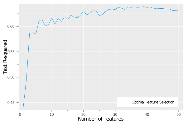
We can see that the model performance grows quickly with the number of features until around 6-8 features are included, at which point the performance seems to level off around 0.61-0.62.
For any given sparsity, we can also investigate which features were selected. For example, we can look at the model with 8 features:
lnr = IAI.OptimalFeatureSelectionRegressor(sparsity=8)
IAI.fit!(lnr, train_X, train_y)
Fitted OptimalFeatureSelectionRegressor:
Constant: 90.4353
Weights:
X0=ak: 5.32555
X0=x: 5.52807
X232: -4.09042
X263: 4.09042
X279: -4.09042
X29: -4.09042
X314: 12.8687
X315: 20.7024From this, we can see that a variety of the features have been selected.
Elastic Net
Next, we will use elastic net regression to conduct the same feature selection exercise and compare the results to Optimal Feature Selection.
The elastic net (and by extension, the lasso) is a method widely used for feature selection and sparsification. However, as shown by Bertsimas and Copenhaver, these methods actually find solutions that are robust to data perturbations, which happen to be naturally sparser than other solutions. Unlike Optimal Feature Selection, these methods do not claim to find the optimal model for a given sparsity, and we will investigate any differences as we compare the methods.
We can fit the elastic net along the entire regularization path using cross-validation with GLMNetCVRegressor:
glmnet_lnr = IAI.GLMNetCVRegressor()
IAI.fit!(glmnet_lnr, train_X, train_y)
For each solution along the regularization path, we will record the sparsity and test performance:
using Statistics: mean
for i = 1:IAI.get_num_fits(glmnet_lnr)
  numeric_weights, categoric_weights = IAI.get_prediction_weights(glmnet_lnr,
                                                                  fit_index=i)
  sparsity = length(numeric_weights) + sum(length.(values(categoric_weights)))
  test_r2 = IAI.score(glmnet_lnr, test_X, test_y, fit_index=i)

  append!(results, DataFrame(
      method="Elastic Net",
      sparsity=sparsity,
      test_r2=test_r2,
  ))
end
sort!(results, [:method, :sparsity])
Method Comparison
Now we can plot and compare the results between the two methods:
using Plots
plot(results.sparsity, results.test_r2,
    group=results.method,
    xlabel="Number of features",
    ylabel="Test R-squared",
    legend=:bottomright,
)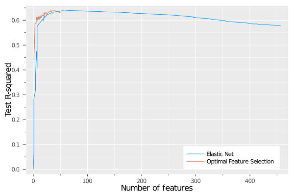
We can see that the elastic net peaks before 100 features, so let's zoom in on this region:
using Plots
plot(results.sparsity, results.test_r2,
    group=results.method,
    xlabel="Number of features",
    ylabel="Test R-squared",
    legend=:bottomright,
    xlim=(0, 100)
)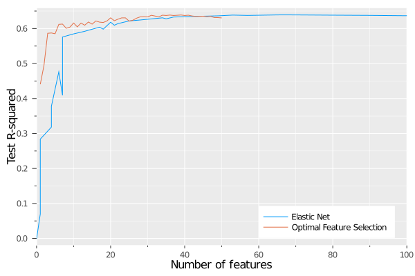
We can see that both methods reach the same level of out-of-sample performance of around 0.62, but there is a significant difference in the number of features needed to attain this performance. As seen earlier, Optimal Feature Selection reaches this level with 6-8 features, whereas the elastic net needs close to 50.
This gives strong evidence to reinforce the earlier point that elastic net and lasso are not designed for feature selection, but rather for robustness. They give sparser solutions than other regularization approaches, but these solutions are not as sparse as they could be. Using Optimal Feature Selection to solve the feature selection problem to optimality gives us the ability to truly explore the tradeoff between model performance and sparsity exactly.