Quick Start Guide: Heuristic Survival Learners
In this example we will use survival learners from Heuristics on the Monoclonal Gammopathy dataset to predict patient survival time (refer to the data preparation guide to learn more about the data format for survival problems). First we load in the data and split into training and test datasets:
using CSV, DataFrames
df = CSV.read("mgus2.csv", DataFrame, missingstring="NA", pool=true)
1384×11 DataFrame
Row │ Column1 id age sex hgb creat mspike ptime ps ⋯
│ Int64 Int64 Int64 String Float64? Float64? Float64? Int64 In ⋯
──────┼─────────────────────────────────────────────────────────────────────────
1 │ 1 1 88 F 13.1 1.3 0.5 30 ⋯
2 │ 2 2 78 F 11.5 1.2 2.0 25
3 │ 3 3 94 M 10.5 1.5 2.6 46
4 │ 4 4 68 M 15.2 1.2 1.2 92
5 │ 5 5 90 F 10.7 0.8 1.0 8 ⋯
6 │ 6 6 90 M 12.9 1.0 0.5 4
7 │ 7 7 89 F 10.5 0.9 1.3 151
8 │ 8 8 87 F 12.3 1.2 1.6 2
⋮ │ ⋮ ⋮ ⋮ ⋮ ⋮ ⋮ ⋮ ⋮ ⋱
1378 │ 1378 1378 56 M 16.1 0.8 0.5 59 ⋯
1379 │ 1379 1379 73 M 15.6 1.1 0.5 48
1380 │ 1380 1380 69 M 15.0 0.8 0.0 22
1381 │ 1381 1381 78 M 14.1 1.3 1.9 35
1382 │ 1382 1382 66 M 12.1 2.0 0.0 31 ⋯
1383 │ 1383 1383 82 F 11.5 1.1 2.3 38
1384 │ 1384 1384 79 M 9.6 1.1 1.7 6
3 columns and 1369 rows omittedX = df[:, 3:(end - 4)]
died = df.death .== 1
times = df.futime
(train_X, train_died, train_times), (test_X, test_died, test_times) =
IAI.split_data(:survival, X, died, times, seed=12345)Random Forest Survival Learner
We will use a GridSearch to fit a RandomForestSurvivalLearner with some basic parameter validation:
grid = IAI.GridSearch(
    IAI.RandomForestSurvivalLearner(
        missingdatamode=:separate_class,
        random_seed=1,
    ),
    max_depth=5:10,
)
IAI.fit!(grid, train_X, train_died, train_times)
All Grid Results:
Row │ max_depth train_score valid_score rank_valid_score
│ Int64 Float64 Float64 Int64
─────┼───────────────────────────────────────────────────────
1 │ 5 0.291592 0.216862 1
2 │ 6 0.310289 0.212261 2
3 │ 7 0.322973 0.206279 3
4 │ 8 0.329134 0.202891 4
5 │ 9 0.331598 0.20266 5
6 │ 10 0.332294 0.202477 6
Best Params:
max_depth => 5
Best Model - Fitted RandomForestSurvivalLearnerWe can make predictions on new data using predict. For survival learners, this returns the appropriate SurvivalCurve for each point, which we can then use to query the mortality probability for any given time t (in this case for t = 10):
pred_curves = IAI.predict(grid, test_X)
t = 10
[c[t] for c in pred_curves]
415-element Vector{Float64}:
0.187396493728
0.212154980723
0.092591201757
0.112061137082
0.215569821689
0.065290983536
0.212558861798
0.183942502458
0.135830805771
0.059289362626
⋮
0.044168066296
0.210253885428
0.087656625803
0.253140933592
0.016125002538
0.102207823668
0.14985600766
0.082458746894
0.175596007719Alternatively, we can get this mortality probability for any given time t by providing t as a keyword argument directly:
IAI.predict(grid, test_X, t=10)415-element Vector{Float64}:
0.187396493728
0.212154980723
0.092591201757
0.112061137082
0.215569821689
0.065290983536
0.212558861798
0.183942502458
0.135830805771
0.059289362626
⋮
0.044168066296
0.210253885428
0.087656625803
0.253140933592
0.016125002538
0.102207823668
0.14985600766
0.082458746894
0.175596007719We can also estimate the survival time for each point:
IAI.predict_expected_survival_time(grid, test_X)415-element Vector{Float64}:
62.960069798779
60.451911795869
128.122472190415
80.415385085702
58.226319438976
135.239279269937
109.304740210212
68.303468814585
133.166596426567
115.056024736284
⋮
182.832081869042
59.377709561932
127.219213341943
86.951384261595
313.631215413167
77.03670255963
56.40262151127
86.157655986924
116.585871130823We can evaluate the quality of the model using score with any of the supported loss functions. For example, the Harrell's c-statistic on the training set:
IAI.score(grid, train_X, train_died, train_times,
criterion=:harrell_c_statistic)0.728648073106186Or on the test set:
IAI.score(grid, test_X, test_died, test_times, criterion=:harrell_c_statistic)0.7130325263974928We can also evaluate the performance of the model at a particular point in time using classification criteria. For instance, we can evaluate the AUC of the 10-month survival predictions on the test set:
IAI.score(grid, test_X, test_died, test_times, criterion=:auc,
evaluation_time=10)0.7750750750750736We can also look at the variable importance:
IAI.variable_importance(IAI.get_learner(grid))5×2 DataFrame
Row │ Feature Importance
│ Symbol Float64
─────┼─────────────────────
1 │ age 0.62681
2 │ hgb 0.187153
3 │ creat 0.109443
4 │ mspike 0.0489006
5 │ sex 0.0276938XGBoost Survival Learner
We will use a GridSearch to fit a XGBoostSurvivalLearner with some basic parameter validation:
grid = IAI.GridSearch(
    IAI.XGBoostSurvivalLearner(
        random_seed=1,
    ),
    max_depth=2:5,
    num_round=[20, 50, 100],
)
IAI.fit!(grid, train_X, train_died, train_times)
All Grid Results:
Row │ num_round max_depth train_score valid_score rank_valid_score
│ Int64 Int64 Float64 Float64 Int64
─────┼──────────────────────────────────────────────────────────────────
1 │ 20 2 0.215788 0.15041 1
2 │ 20 3 0.194945 -0.0670846 3
3 │ 20 4 0.183779 -0.121177 4
4 │ 20 5 0.0916703 -0.401915 7
5 │ 50 2 0.210932 0.0262287 2
6 │ 50 3 0.153306 -0.217315 6
7 │ 50 4 0.0281118 -0.513705 9
8 │ 50 5 -0.180287 -0.874789 10
9 │ 100 2 0.182667 -0.132212 5
10 │ 100 3 0.0250015 -0.512681 8
11 │ 100 4 -0.345342 -1.03887 11
12 │ 100 5 -0.907832 -1.75591 12
Best Params:
num_round => 20
max_depth => 2
Best Model - Fitted XGBoostSurvivalLearnerWe can make predictions on new data using predict. For survival learners, this returns the appropriate SurvivalCurve for each point, which we can then use to query the mortality probability for any given time t (in this case for t = 10):
pred_curves = IAI.predict(grid, test_X)
t = 10
[c[t] for c in pred_curves]
415-element Vector{Float64}:
0.14218
0.19365
0.10101
0.21149
0.21305
0.06571
0.11277
0.13989
0.09729
0.06921
⋮
0.04348
0.14986
0.08444
0.14099
0.01246
0.1504
0.21825
0.12885
0.22829Alternatively, we can get this mortality probability for any given time t by providing t as a keyword argument directly:
IAI.predict(grid, test_X, t=10)415-element Vector{Float64}:
0.14218
0.19365
0.10101
0.21149
0.21305
0.06571
0.11277
0.13989
0.09729
0.06921
⋮
0.04348
0.14986
0.08444
0.14099
0.01246
0.1504
0.21825
0.12885
0.22829We can also estimate the survival time for each point:
IAI.predict_expected_survival_time(grid, test_X)415-element Vector{Float64}:
103.14
73.356
143.604
66.184
65.612
200.331
129.869
104.9
148.39
193.413
⋮
253.328
97.563
166.9
104.048
363.12
97.19
63.766
114.09
60.43We can evaluate the quality of the model using score with any of the supported loss functions. For example, the Harrell's c-statistic on the training set:
IAI.score(grid, train_X, train_died, train_times,
criterion=:harrell_c_statistic)0.71899034Or on the test set:
IAI.score(grid, test_X, test_died, test_times, criterion=:harrell_c_statistic)0.70912965We can also evaluate the performance of the model at a particular point in time using classification criteria. For instance, we can evaluate the AUC of the 10-month survival predictions on the test set:
IAI.score(grid, test_X, test_died, test_times, criterion=:auc,
evaluation_time=10)0.68960961We can also look at the variable importance:
IAI.variable_importance(IAI.get_learner(grid))5×2 DataFrame
Row │ Feature Importance
│ Symbol Float64
─────┼─────────────────────
1 │ age 0.427724
2 │ creat 0.200167
3 │ hgb 0.154691
4 │ sex=M 0.115374
5 │ mspike 0.102045We can calculate the SHAP values:
s = IAI.predict_shap(grid, test_X)
s[:shap_values]
415×5 Matrix{Float64}:
0.61058 0.30582 -0.04894 -0.01826 -0.14742
1.07476 0.16585 -0.04894 -0.00356 -0.14742
0.23345 0.18522 0.05296 -0.01366 -0.12105
1.4023 -0.05959 -0.05695 -0.01366 -0.13249
0.69856 0.2627 0.04495 -0.02039 0.16211
0.18722 -0.14855 -0.04093 -0.00356 -0.10612
-0.18245 0.42472 0.12438 -0.01668 0.10355
0.77792 0.12435 -0.05695 -0.01366 -0.14742
0.13403 0.33627 -0.03813 -0.01366 -0.12105
0.24808 -0.14301 -0.04354 -0.01366 -0.10612
⋮
-0.38698 -0.15637 -0.05912 -0.01668 0.08266
0.63852 0.2364 0.04495 -0.01366 -0.14742
0.15582 -0.16502 0.05296 -0.00568 0.11068
-0.39859 0.50849 0.43877 0.32741 -0.18338
-1.78685 -0.19225 0.18891 -0.08385 0.07211
0.73717 -0.14956 0.03954 -0.00568 0.14121
1.07879 -0.07867 0.03954 -0.00568 0.14121
0.6234 -0.16209 0.03954 -0.01578 0.11068
-0.26166 0.29492 0.19171 0.81775 0.18365We can then use the SHAP library in Python to visualize these results in whichever way we prefer. For example, the following code creates a summary plot:
using PyCall
shap = pyimport("shap")
shap.summary_plot(s[:shap_values], Matrix(s[:features]), names(s[:features]))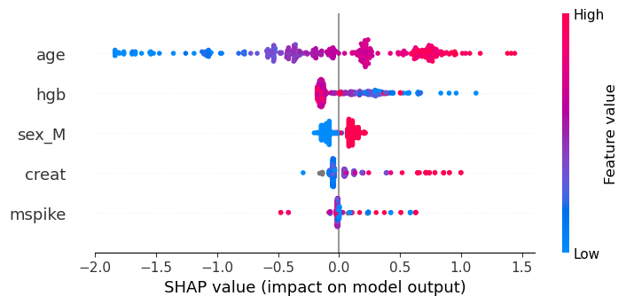
GLMNetCV Survival Learner
We will fit a GLMNetCVSurvivalLearner directly. Since GLMNetCVLearner does not support missing data, we first subset to complete cases:
train_cc = completecases(train_X)
train_X_cc = train_X[train_cc, :]
train_died_cc = train_died[train_cc]
train_times_cc = train_times[train_cc]

test_cc = completecases(test_X)
test_X_cc = test_X[test_cc, :]
test_died_cc = test_died[test_cc]
test_times_cc = test_times[test_cc]
We can now proceed with fitting the learner:
lnr = IAI.GLMNetCVSurvivalLearner(random_seed=1)
IAI.fit!(lnr, train_X_cc, train_died_cc, train_times_cc)
Fitted GLMNetCVSurvivalLearner:
Constant: -3.319
Weights:
age: 0.0578244
creat: 0.18159
hgb: -0.0889831
sex=M: 0.300142We can make predictions on new data using predict. For survival learners, this returns the appropriate SurvivalCurve for each point, which we can then use to query the mortality probability for any given time t (in this case for t = 10):
pred_curves = IAI.predict(lnr, test_X_cc)
t = 10
[c[t] for c in pred_curves]
401-element Vector{Float64}:
0.200607896718
0.370165075078
0.122585629449
0.258150249738
0.263183570494
0.097649876452
0.130211918883
0.165323978367
0.142078644844
0.115488054643
⋮
0.288921901855
0.077102775305
0.225010337685
0.132377147815
0.032757577054
0.310343253654
0.295608518778
0.191789512261
0.123660862616Alternatively, we can get this mortality probability for any given time t by providing t as a keyword argument directly:
IAI.predict(lnr, test_X_cc, t=10)401-element Vector{Float64}:
0.200607896718
0.370165075078
0.122585629449
0.258150249738
0.263183570494
0.097649876452
0.130211918883
0.165323978367
0.142078644844
0.115488054643
⋮
0.288921901855
0.077102775305
0.225010337685
0.132377147815
0.032757577054
0.310343253654
0.295608518778
0.191789512261
0.123660862616We can also estimate the survival time for each point:
IAI.predict_expected_survival_time(lnr, test_X_cc)401-element Vector{Float64}:
69.71314448
32.21543141
118.46926932
51.54736223
50.33089515
146.17629908
111.58709637
86.76397257
102.05616823
125.48250448
⋮
44.76791753
176.94796956
60.89939196
109.74632954
283.63478532
40.83477821
43.47980691
73.42616111
117.45965404We can evaluate the quality of the model using score with any of the supported loss functions. For example, the Harrell's c-statistic on the training set:
IAI.score(lnr, train_X_cc, train_died_cc, train_times_cc,
criterion=:harrell_c_statistic)0.6837433757104808Or on the test set:
IAI.score(lnr, test_X_cc, test_died_cc, test_times_cc,
criterion=:harrell_c_statistic)0.7027583847744624We can also evaluate the performance of the model at a particular point in time using classification criteria. For instance, we can evaluate the AUC of the 10-month survival predictions on the test set:
IAI.score(lnr, test_X_cc, test_died_cc, test_times_cc, criterion=:auc,
evaluation_time=10)0.6823274764451254We can also look at the variable importance:
IAI.variable_importance(lnr)5×2 DataFrame
Row │ Feature Importance
│ Symbol Float64
─────┼─────────────────────
1 │ age 0.59208
2 │ hgb 0.153895
3 │ sex=M 0.127414
4 │ creat 0.12661
5 │ mspike 0.0