Quick Start Guide: Optimal Feature Selection for Regression
This is a Python version of the corresponding OptimalFeatureSelection quick start guide.
In this example we will use Optimal Feature Selection on the Ailerons dataset, which addresses a control problem, namely flying a F16 aircraft. The attributes describe the status of the aeroplane, while the goal is to predict the control action on the ailerons of the aircraft.
First we load in the data and split into training and test datasets:
import pandas as pd
df = pd.read_csv("ailerons.csv")
       climbRate  Sgz     p     q  ...  diffSeTime14  alpha     Se    goal
0              2  -56 -0.33 -0.09  ...           0.0    0.9  0.032 -0.0009
1            470  -39  0.02  0.12  ...           0.0    0.9  0.034 -0.0011
2            165    4  0.14  0.14  ...           0.0    1.0  0.034 -0.0012
3           -113    5 -0.12  0.11  ...           0.0    0.9  0.033 -0.0011
4           -411  -21 -0.17  0.07  ...           0.0    0.9  0.032 -0.0008
5           -105  -42  0.23 -0.06  ...           0.0    0.8  0.028 -0.0010
6            144  -40  0.31 -0.01  ...           0.0    0.8  0.029 -0.0012
...          ...  ...   ...   ...  ...           ...    ...    ...     ...
13743       -224  -24 -0.22  0.00  ...           0.0    0.7  0.026 -0.0007
13744       -204  -27 -0.25  0.01  ...           0.0    0.7  0.026 -0.0006
13745        399  -22  0.17  0.20  ...           0.0    0.8  0.027 -0.0008
13746        237   -6  0.26  0.10  ...           0.0    0.8  0.027 -0.0010
13747       -148   -3 -0.37  0.09  ...           0.0    0.7  0.026 -0.0006
13748       -237  -11 -0.47 -0.16  ...           0.0    0.7  0.023 -0.0005
13749        128  -14 -0.07 -0.11  ...           0.0    0.6  0.022 -0.0006

[13750 rows x 41 columns]
from interpretableai import iai
X = df.iloc[:, 0:-1]
y = df.iloc[:, -1]
(train_X, train_y), (test_X, test_y) = iai.split_data('regression', X, y, seed=1)
Model Fitting
We will use a GridSearch to fit an OptimalFeatureSelectionRegressor:
grid = iai.GridSearch(
    iai.OptimalFeatureSelectionRegressor(
        random_seed=1,
    ),
    sparsity=range(1, 11),
)
grid.fit(train_X, train_y)
All Grid Results:

 Row │ sparsity  train_score  valid_score  rank_valid_score
     │ Int64     Float64      Float64      Int64
─────┼──────────────────────────────────────────────────────
   1 │        1     0.49788      0.475188                10
   2 │        2     0.663576     0.668303                 9
   3 │        3     0.749368     0.752557                 8
   4 │        4     0.807263     0.804385                 7
   5 │        5     0.812985     0.808196                 6
   6 │        6     0.816881     0.810463                 5
   7 │        7     0.818946     0.813062                 3
   8 │        8     0.818662     0.812035                 4
   9 │        9     0.819254     0.813463                 1
  10 │       10     0.819036     0.81332                  2

Best Params:
  sparsity => 9

Best Model - Fitted OptimalFeatureSelectionRegressor:
  Constant: 0.000345753
  Weights:
    SeTime1:      -0.00703259
    SeTime2:      -0.00948655
    SeTime3:      -0.00954495
    Sgz:           0
    absRoll:       0.0000576494
    curRoll:      -0.0000862381
    diffClb:      -0.00000279116
    diffRollRate:  0.00253189
    p:            -0.000425322
The model selected a sparsity of 9 as the best parameter, but we observe that the validation scores are close for many of the parameters. We can use the results of the grid search to explore the tradeoff between the complexity of the regression and the quality of predictions:
grid.plot(type='validation')
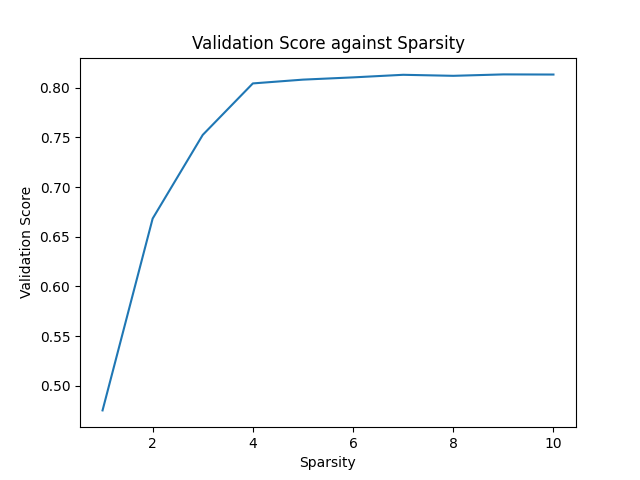
We see that the quality of the model quickly increases with additional terms until we reach 4, and then only small increases afterwards. Depending on the application, we might decide to choose a lower sparsity for the final model than the value chosen by the grid search.
We can see the relative importance of the selected features with variable_importance:
grid.get_learner().variable_importance()
Feature Importance
0 absRoll 0.340282
1 p 0.184247
2 curRoll 0.119241
3 SeTime3 0.094151
4 SeTime2 0.093578
5 SeTime1 0.069062
6 diffRollRate 0.048109
.. ... ...
33 diffSeTime4 0.000000
34 diffSeTime5 0.000000
35 diffSeTime6 0.000000
36 diffSeTime7 0.000000
37 diffSeTime8 0.000000
38 diffSeTime9 0.000000
39 q 0.000000
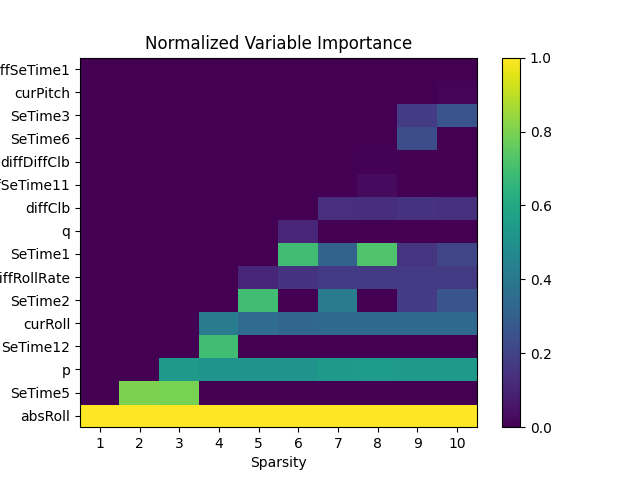
[40 rows x 2 columns]We can also look at the feature importance across all sparsity levels:
grid.plot(type='importance')
We can make predictions on new data using predict:
grid.predict(test_X)
array([-0.00103828, -0.00124997, -0.00120794, ..., -0.00121972,
       -0.00077037, -0.00097959])
We can evaluate the quality of the model using score with any of the supported loss functions. For example, the $R^2$ on the training set:
grid.score(train_X, train_y, criterion='mse')
0.817629588096Or on the test set:
grid.score(test_X, test_y, criterion='mse')
0.817330661094