Quick Start Guide: Optimal Feature Selection for Classification
In this example we will use optimal feature selection on the Mushroom dataset, where the goal is to distinguish poisonous from edible mushrooms.
First we load in the data and split into training and test datasets:
using CSV, DataFrames
df = CSV.read("agaricus-lepiota.data", DataFrame,
    pool=true,
    header=[:target, :cap_shape, :cap_surface, :cap_color, :bruises, :odor,
            :gill_attachment, :gill_spacing, :gill_size, :gill_color,
            :stalk_shape, :stalk_root, :stalk_surface_above,
            :stalk_surface_below, :stalk_color_above, :stalk_color_below,
            :veil_type, :veil_color, :ring_number, :ring_type, :spore_color,
            :population, :habitat],
)
8124×23 DataFrame
Row │ target cap_shape cap_surface cap_color bruises odor gill_attac ⋯
│ String String String String String String String ⋯
──────┼─────────────────────────────────────────────────────────────────────────
1 │ p x s n t p f ⋯
2 │ e x s y t a f
3 │ e b s w t l f
4 │ p x y w t p f
5 │ e x s g f n f ⋯
6 │ e x y y t a f
7 │ e b s w t a f
8 │ e b y w t l f
⋮ │ ⋮ ⋮ ⋮ ⋮ ⋮ ⋮ ⋮ ⋱
8118 │ p k s e f y f ⋯
8119 │ p k y n f f f
8120 │ e k s n f n a
8121 │ e x s n f n a
8122 │ e f s n f n a ⋯
8123 │ p k y n f y f
8124 │ e x s n f n a
17 columns and 8109 rows omittedX = df[:, 2:end]
y = df.target
(train_X, train_y), (test_X, test_y) = IAI.split_data(:classification, X, y,
seed=1)Model Fitting
We will use a GridSearch to fit an OptimalFeatureSelectionClassifier:
grid = IAI.GridSearch(
    IAI.OptimalFeatureSelectionClassifier(
        random_seed=1,
    ),
    sparsity=1:10,
)
IAI.fit!(grid, train_X, train_y, validation_criterion=:auc)
All Grid Results:
Row │ sparsity train_score valid_score rank_valid_score
│ Int64 Float64 Float64 Int64
─────┼──────────────────────────────────────────────────────
1 │ 1 0.530592 0.883816 10
2 │ 2 0.666962 0.958933 9
3 │ 3 0.852881 0.97677 8
4 │ 4 0.886338 0.989837 6
5 │ 5 0.8786 0.989776 7
6 │ 6 0.918052 0.999586 4
7 │ 7 0.921551 0.999586 5
8 │ 8 0.930723 0.999783 1
9 │ 9 0.933428 0.999783 2
10 │ 10 0.933968 0.999755 3
Best Params:
sparsity => 8
Best Model - Fitted OptimalFeatureSelectionClassifier:
Constant: -0.102149
Weights:
gill_color=b: 1.30099
gill_size=n: 2.15205
odor=a: -3.56147
odor=f: 2.41679
odor=l: -3.57161
odor=n: -3.58869
spore_color=r: 6.1136
stalk_surface_above=k: 1.56583
(Higher score indicates stronger prediction for class `p`)The model selected a sparsity of 8 as the best parameter, but we observe that the validation scores are close for many of the parameters. We can use the results of the grid search to explore the tradeoff between the complexity of the regression and the quality of predictions:
using Plots
plot(grid, type=:validation)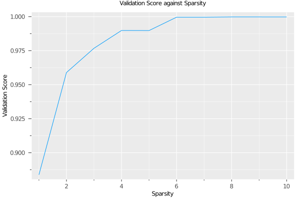
We see that the quality of the model quickly increases with as features are adding, reaching AUC 0.98 with 3 features. After this, additional features increase the quality more slowly, eventually reaching AUC close to 1 with 6 features. Depending on the application, we might decide to choose a lower sparsity for the final model than the value chosen by the grid search.
We can see the relative importance of the selected features with variable_importance:
IAI.variable_importance(IAI.get_learner(grid))112×2 DataFrame
Row │ Feature Importance
│ Symbol Float64
─────┼───────────────────────────────────
1 │ odor=n 0.247412
2 │ odor=f 0.148001
3 │ gill_size=n 0.138891
4 │ odor=l 0.109303
5 │ odor=a 0.105547
6 │ stalk_surface_above=k 0.0986795
7 │ spore_color=r 0.0778057
8 │ gill_color=b 0.0743607
⋮ │ ⋮ ⋮
106 │ stalk_surface_below=s 0.0
107 │ stalk_surface_below=y 0.0
108 │ veil_color=n 0.0
109 │ veil_color=o 0.0
110 │ veil_color=w 0.0
111 │ veil_color=y 0.0
112 │ veil_type=p 0.0
97 rows omittedWe can also look at the feature importance across all sparsity levels:
plot(grid, type=:importance)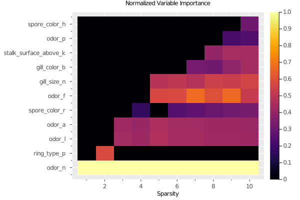
We can make predictions on new data using predict:
IAI.predict(grid, test_X)2437-element Vector{String}:
"e"
"e"
"e"
"e"
"e"
"e"
"e"
"p"
"e"
"e"
⋮
"e"
"p"
"e"
"e"
"p"
"p"
"p"
"p"
"e"We can evaluate the quality of the model using score with any of the supported loss functions. For example, the misclassification on the training set:
IAI.score(grid, train_X, train_y, criterion=:misclassification)0.9982416036574644Or the AUC on the test set:
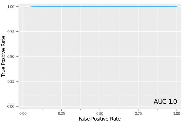
IAI.score(grid, test_X, test_y, criterion=:auc)0.9997835249688102We can plot the ROC curve on the test set as an interactive visualization:
roc = IAI.ROCCurve(grid, test_X, test_y, positive_label="p")We can also plot the same ROC curve as a static image:
plot(roc)