Predicting Risk of Loan Default
In this example, we use the dataset from the FICO Explainable Machine Learning Challenge to compare the performance of Optimal Trees to XGBoost, and also compare the interpretability of the resulting trees to LIME and SHAP, two approaches for model explainability (for additional comparison between interpretability and explainability, you may like to refer to our paper comparing these approaches in the context of feature selection).
The challenge used a dataset of home equity line of credit (HELOC) applications made by real homeowners. A HELOC is a line of credit typically offered by a bank as a percentage of home equity (the difference between the current market value of a home and its purchase price). The customers in this dataset have requested a credit line, and the fundamental task is to use the information about the applicant in their credit report to predict whether they will repay their HELOC account within 2 years. This prediction is then used to decide whether the homeowner qualifies for a line of credit and, if so, how much credit should be extended.
Due to the financial nature of the dataset, FICO posed the challenge of generating high-quality, explainable predictions using this data. When a credit decision is made, the consumer is entitled by regulations to an explanation for any adverse decisions, and thus model interpretability is a must-have for any AI solution to be used in this space.
In this example, we are not going to give great attention to tuning either method for performance, we will just conduct some very rough parameter tuning to give reasonable models for interpretation.
Data Preparation
Read in the data, treating -8 (No Usable/Valid Trade or Inquiry) and -9 (No Record) as missing:
using CSV, DataFrames
df = CSV.read("heloc.csv", DataFrame, missingstring=["-9", "-8"])
10459×24 DataFrame
Row │ RiskPerformance ExternalRiskEstimate MSinceOldestTradeOpen MSinceM ⋯
│ String Int64? Int64? Int64? ⋯
───────┼────────────────────────────────────────────────────────────────────────
1 │ Bad 55 144 ⋯
2 │ Bad 61 58
3 │ Bad 67 66
4 │ Bad 66 169
5 │ Bad 81 333 ⋯
6 │ Bad 59 137
7 │ Good 54 88
8 │ Good 68 148
⋮ │ ⋮ ⋮ ⋮ ⋱
10453 │ Good 90 197 ⋯
10454 │ Bad 75 410
10455 │ Good 73 131
10456 │ Bad 65 147
10457 │ Bad 74 129 ⋯
10458 │ Bad 72 234
10459 │ Bad 66 28
21 columns and 10444 rows omittedDelete 588 rows where all features are missing:
inds = findall(i -> !all(ismissing.(values(df[i, 2:end]))), 1:nrow(df))
df = df[inds, :]
There are two ordinal features in the data, which we will tidy up by converting numeric codes to strings and then encoding as an ordered CategoricalVector:
df.MaxDelq2PublicRecLast12M = map(df.MaxDelq2PublicRecLast12M) do x
    if x == 0
        "Derogatory Comment"
    elseif x == 1
        "120+ Days Delinquent"
    elseif x == 2
        "90 Days Delinquent"
    elseif x == 3
        "60 Days Delinquent"
    elseif x == 4
        "30 Days Delinquent"
    elseif x == 7
        "Never Delinquent"
    else
        missing
    end
end
df.MaxDelqEver = map(df.MaxDelqEver) do x
    if x == 2
        "Derogatory Comment"
    elseif x == 3
        "120+ Days Delinquent"
    elseif x == 4
        "90 Days Delinquent"
    elseif x == 5
        "60 Days Delinquent"
    elseif x == 6
        "30 Days Delinquent"
    elseif x == 8
        "Never Delinquent"
    else
        missing
    end
end

using CategoricalArrays
for col in (:MaxDelq2PublicRecLast12M, :MaxDelqEver)
  df[!, col] = CategoricalVector(df[!, col], ordered=true, levels=[
      "Never Delinquent",
      "30 Days Delinquent",
      "60 Days Delinquent",
      "90 Days Delinquent",
      "120+ Days Delinquent",
      "Derogatory Comment",
  ])
end
There are two numeric columns with an additional special value -7 (Condition not Met). We will treat these as mixed numeric/categoric features:
for colname in [:MSinceMostRecentDelq, :MSinceMostRecentInqexcl7days]
    col = replace(df[!, colname], -7 => "Condition not Met")
    df[!, colname] = IAI.make_mixed_data(col)
end
With all manipulation complete, we split data into training and test sets:
X = df[:, 2:end]
y = df[:, 1]
seed = 12321
(train_X, train_y), (test_X, test_y) = IAI.split_data(:classification, X, y,
                                                      seed=seed)
Optimal Trees
Our first approach to predicting loan defaults is using Optimal Trees. We fit an optimal tree model, validating over the depth of the tree.
grid = IAI.GridSearch(
    IAI.OptimalTreeClassifier(
        missingdatamode=:separate_class,
        random_seed=seed,
    ),
    max_depth=4:6,
)
IAI.fit_cv!(grid, train_X, train_y, validation_criterion=:auc, n_folds=5)
lnr = IAI.get_learner(grid)
IAI.set_display_label!(lnr, "Bad")We can evaluate the out-of-sample performance:
IAI.score(grid, test_X, test_y, criterion=:misclassification)0.724510465901418IAI.score(grid, test_X, test_y, criterion=:auc)0.7454765611406909Model Interpretation
The tree visualization can easily be inspected to examine the transparent logic behind the predictions made by the tree. It is also possible to combine the tree visualization with the underlying data so that you can interactively explore the predictions of the tree. To do this, we simply pass the data keyword argument to write_html:
IAI.write_html("tree_with_data.html", lnr, data=(X, y))The resulting interactive visualization can be viewed here, refer to the documentation on tree visualizations for more information.
You can also examine the path through the tree for any point using the print_path function. Here, we look at the explanation for the first point:
IAI.print_path(lnr, test_X, 1)Rules used to predict sample 1:
1) Split: NumSatisfactoryTrades (=25) < 27.5
2) Split: MSinceMostRecentInqexcl7days (=0) is Condition not Met or < 0.5
3) Split: ExternalRiskEstimate (=54) < 74.5
4) Predict: Bad (P(Bad) = 78.18%), [1756,490], 2246 points, error 0.2182We can see that the first sample is predicted as an 78% risk of being a bad loan because:
- the number of satisfactory tradelines is 25, lower than the threshold of 27.5, increasing the risk;
- the number of months since the most recent inquiry was 0, below the threshold of 0.5; increasing the risk;
- the external risk score estimate of 54 is below the threshold of 74.5, increasing the risk;
- there are 2246 loans in the training set similar to this given point, based on satisfying these criteria, and 1756 (78%) of these were bad.
We can summarize these conditions to conclude that applicants with an external risk score of 74 or lower, less than one month since the last credit inquiry, and fewer than 28 satisfactory tradelines have a 78% chance of being a bad loan. This is a succinct, straightforward and understandable justification for the prediction being made, and only uses three of the features in the dataset to make this choice.
XGBoost with LIME/Shap
Next, we are going to use XGBoost to make predictions on the data, and then use LIME and SHAP to generate explanations for these predictions.
Data Preparation
LIME and SHAP are implemented in Python, so we are going to call these from Julia using PyCall.jl, which makes it easy to access Python libraries inside Julia.
XGBoost does not support the mixed-data encoding we used for Optimal Trees, so we need to re-encode the mixed data. First, we undo the mixed data transformation so that we can pass the data to Python:
for col in (:MSinceMostRecentDelq, :MSinceMostRecentInqexcl7days)
  df[!, col] = IAI.undo_mixed_data(df[!, col])
end
We will also convert the ordinal variables back to numbers so that XGBoost can work with them directly:
df.MaxDelq2PublicRecLast12M = map(df.MaxDelq2PublicRecLast12M) do x
  if ismissing(x)
    missing
  elseif x == "Derogatory Comment"
    0
  elseif x == "120+ Days Delinquent"
    1
  elseif x == "90 Days Delinquent"
    2
  elseif x == "60 Days Delinquent"
    3
  elseif x == "30 Days Delinquent"
    4
  elseif x == "Never Delinquent"
    7
  end
end
df.MaxDelqEver = map(df.MaxDelqEver) do x
  if ismissing(x)
    missing
  elseif x == "Derogatory Comment"
    2
  elseif x == "120+ Days Delinquent"
    3
  elseif x == "90 Days Delinquent"
    4
  elseif x == "60 Days Delinquent"
    5
  elseif x == "30 Days Delinquent"
    6
  elseif x == "Never Delinquent"
    8
  end
end
We encode the labels as integers to work with XGBoost:
df.RiskPerformance = Int.(df.RiskPerformance .== "Good")As mentioned above, we will be doing the model fitting and interpretation in Python via PyCall.jl, so we will first convert the data to a Pandas DataFrame by saving the data to CSV and loading it Pandas:
CSV.write("train_df.csv", df[train_y.indices[1], :])
CSV.write("test_df.csv", df[test_y.indices[1], :])

using PyCall
pd = pyimport("pandas")
function load_data(filename)
    df = pd.read_csv(filename)
    y = df.RiskPerformance
    X = df.drop(["RiskPerformance"], axis=1)
    return X, y
end

train_X, train_y = load_data("train_df.csv")
test_X, test_y = load_data("test_df.csv")
Now we handle the columns that were mixed data in Julia. We use the weight-of-evidence (WoE) encoding to represent the column with numeric values.
ce = pyimport("category_encoders")
encoder = ce.WOEEncoder(cols=["MSinceMostRecentInqexcl7days",
                              "MSinceMostRecentDelq"])
train_X = encoder.fit_transform(train_X, train_y)
test_X = encoder.transform(test_X)
Model Fitting
With the data prepared, we can fit an XGBoost model, validating over the depth:
xgboost = pyimport("xgboost.sklearn")
model_selection = pyimport("sklearn.model_selection")
xgb = model_selection.GridSearchCV(
    xgboost.XGBClassifier(
        seed=seed,
    ),
    Dict("max_depth" => 2:8),
    cv=5,
)
xgb.fit(train_X.values, train_y)
We can then evaluate the out-of-sample performance:
pred_y = xgb.predict(test_X.values)
metrics = pyimport("sklearn.metrics")
metrics.accuracy_score(test_y, pred_y)0.7292370020256583metrics.roc_auc_score(test_y, xgb.predict_proba(test_X.values)[:, 2])0.7950073090168288Model Interpretation
Now that we have a trained black-box model, we can investigate the approaches for explaining its predictions. We will focus on the same sample point used above with Optimal Trees:
xgb.predict_proba(test_X.values)[1, :]2-element Vector{Float32}:
0.9336462
0.0663538We see that the predicted probability of default for this point under the XGBoost model is 93%, which is in line with the high risk of default predicted by the Optimal Trees model.
LIME
First we use LIME to explain the prediction for a single row at a time. LIME (local interpretable model-agnostic explanations) is an explanation technique that explains the predictions of a classifier by learning a linear model locally around the prediction.
Here we show the explanation for the same sample point as above:
lime = pyimport("lime.lime_tabular")
lime_explainer = lime.LimeTabularExplainer(
    train_X.astype("float"),
    feature_names=train_X.columns,
    class_names=["Bad", "Good"],
    discretize_continuous=false,
    random_state=1,
)
explanation = lime_explainer.explain_instance(test_X.iloc[1].values,
                                              xgb.predict_proba)
explanation.as_pyplot_figure()
Lime attempts to explain the local sensitivity of the prediction to the features in the dataset. Here it tells us that the three most significant factors in the prediction for this point are the time since the most recent delinquency, the external risk estimate, and the time since the most recent inquiry (and increasing each of these values will push the prediction towards Good).
We see that the features that were used by the tree prediction show up among these significant factors, but many more than these are included, complicating the interpretation.
Another limitation of the LIME explanation is that it is only local in nature, telling us how the current prediction will change in response to small changes in the input values. It therefore behaves more like a sensitivity analysis rather than an explanation for why the prediction was made in the first place.
SHAP
Next we will generate model explanations using SHAP. SHAP is an approach to explain the output of any machine learning model by assigning each feature in the data an importance value for every prediction made:
shap = pyimport("shap")
shap_explainer = shap.TreeExplainer(xgb.best_estimator_)
shap_values = shap_explainer.shap_values(test_X)
First we generate a summary plot, that shows the overall importance of the features in the dataset according to the SHAP values
shap.summary_plot(shap_values, test_X)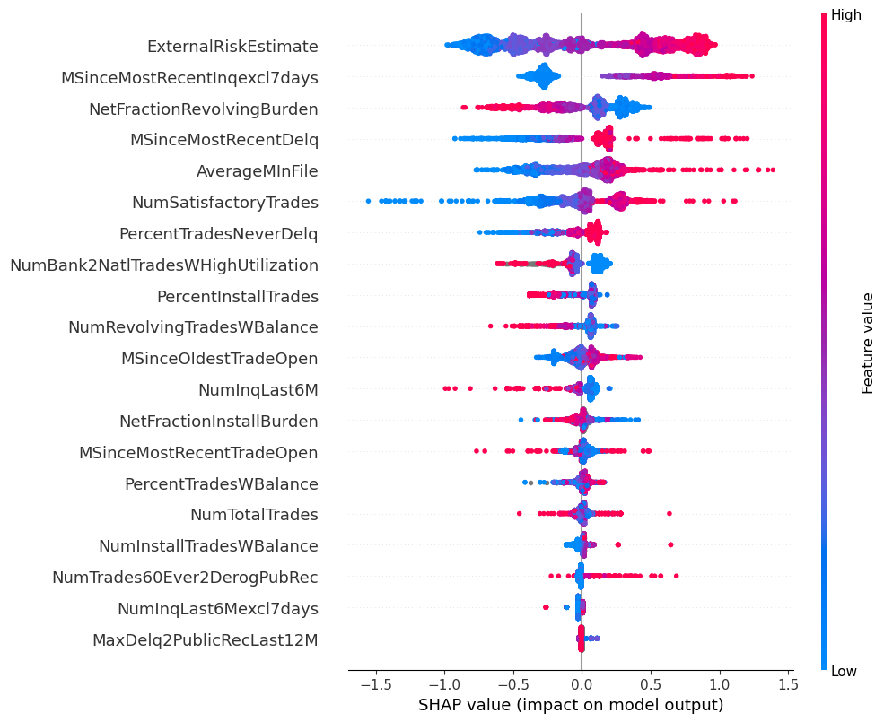
This shows us the relative importance of the features in the model overall, and we can see the features with more impact are generally also the ones that were used by the tree.
We can also look at the variation of the SHAP values as the value of a single feature in the dataset changes:
shap.dependence_plot("ExternalRiskEstimate", shap_values, test_X,
                     interaction_index="MSinceMostRecentInqexcl7days")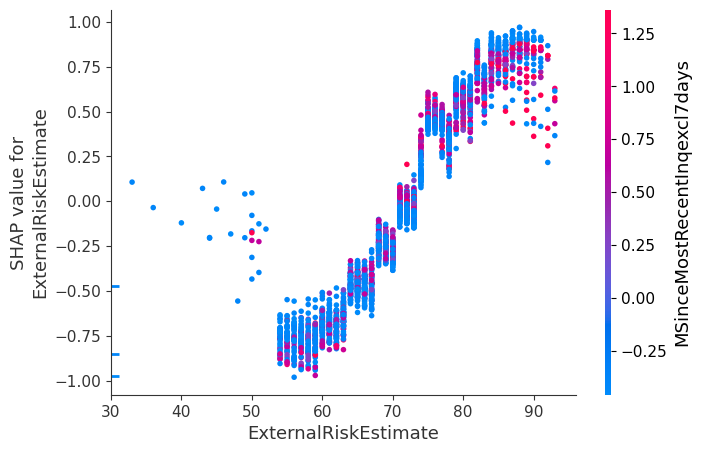
This plot shows us that the external risk estimate is largely linearly correlated with its impact on the predicted outcome. From the color scale, the plot shows there is no interaction effect between the external risk estimate and the time since the most recent inquiry, as the trend in the plot is independent of color (despite the time affecting the external risk score). In comparison, by inspecting the trees output, we see that there are signs of interactions between these two variables as they are both used in different locations of the tree with different thresholds each time, indicating that each feature's importance to predictions might be dependent on the value of the other.
These previous plots were summarizing aggregate effects, showing how the features are related on average to the predictions. We can also use the SHAP values to investigate the prediction made for a single point (using the same single point as earlier for Optimal Trees and LIME):
shap.force_plot(shap_explainer.expected_value, shap_values[1, :],
                test_X.iloc[1], matplotlib=true)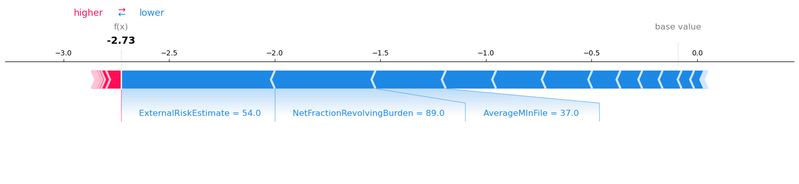
We see that from the SHAP explanation that the most significant feature pushing the prediction towards Bad is the external risk estimate. This is followed by the utilization of revolving credit lines and the average age of the credit file. There are over ten additional features with importances assigned in the explanation, pushing the prediction in both directions.
Note that the time since the most recent inquiry is not one of the most important factors. This is unlike in the LIME explanation where it was one of the three most important features, and in the optimal tree model where it was one of three relevant factors alongside the external risk estimate and the number of satisfactory tradelines. This is again evidence that this approach to explanation may have trouble isolating the interactions between variables to succinctly interpret the model output.
Conclusions
In this example, we compared two approaches for predicting loan defaults and interpreting the resulting model. The logic behind the optimal tree model and its predictions is transparent and clear. In contrast, the LIME and SHAP explanations assigned importance to the features used by the tree, but also to many others, making it harder to construct a succinct description of the prediction mechanism. In the example prediction we attempted to explain, LIME assigned importance to the same features used by the tree, among many others, while SHAP did not assign much importance to one of these features at all.